
Sys.time()[1] "2023-08-12 07:28:04 CDT"Sys.time()[1] "2023-08-12 07:28:04 CDT"[1] "America/Chicago"PROJECT_DIR <- file.path(
"/Users/jialei/Dropbox/Data/Projects/UTSW",
"/Cardiomyopathy/atac-seq"
)Load required packages.
library(tidyverse)
## ── Attaching core tidyverse packages ─────────────────── tidyverse 2.0.0.9000 ──
## ✔ dplyr     1.1.2.9000     ✔ readr     2.1.4.9000
## ✔ forcats   1.0.0.9000     ✔ stringr   1.5.0.9000
## ✔ ggplot2   3.4.2.9000     ✔ tibble    3.2.1.9005
## ✔ lubridate 1.9.2.9000     ✔ tidyr     1.3.0.9000
## ✔ purrr     1.0.2.9000
## ── Conflicts ────────────────────────────────────────── tidyverse_conflicts() ──
## ✖ dplyr::filter() masks stats::filter()
## ✖ dplyr::lag()    masks stats::lag()
## ℹ Use the conflicted package (<http://conflicted.r-lib.org/>) to force all conflicts to become errors
library(Matrix)
##
## Attaching package: 'Matrix'
##
## The following objects are masked from 'package:tidyr':
##
##     expand, pack, unpack
library(patchwork)
library(extrafont)
## Registering fonts with R`%+replace%` <- ggplot2::`%+replace%`numpy version: 1.24.3 reticulate::py_config()python: /Users/jialei/.pyenv/shims/python
libpython: /Users/jialei/.pyenv/versions/mambaforge-22.9.0-3/lib/libpython3.10.dylib
pythonhome: /Users/jialei/.pyenv/versions/mambaforge-22.9.0-3:/Users/jialei/.pyenv/versions/mambaforge-22.9.0-3
version: 3.10.9 | packaged by conda-forge | (main, Feb 2 2023, 20:26:08) [Clang 14.0.6 ]
numpy: /Users/jialei/.pyenv/versions/mambaforge-22.9.0-3/lib/python3.10/site-packages/numpy
numpy_version: 1.24.3
numpy: /Users/jialei/.pyenv/versions/mambaforge-22.9.0-3/lib/python3.10/site-packages/numpy
NOTE: Python version was forced by RETICULATE_PYTHONfs::dir_ls(
path = file.path(
PROJECT_DIR,
"qc",
"tss_enrichment/raw/core_set_merged",
"cut_site"
),
regexp = "npy$"
) |>
purrr::map(\(x) {
np$load(file = x) |>
{
\(y) {
y / mean(c(y[1:100], y[4102:4201]))
}
}() |>
tibble::enframe(name = "position", value = "score") |>
dplyr::mutate(
category = x |>
basename() |>
stringr::str_remove(
pattern = "Aligned_sorted_deduped_q10_"
) |>
stringr::str_remove(
pattern = "_21_tss_flanking_0.npy"
)
)
}) |>
dplyr::bind_rows() |>
dplyr::mutate(
category = category |> stringr::str_to_title(),
category = dplyr::case_when(
category == "Fresh_healthy" ~ "Healthy",
category == "Fresh_icm" ~ "ICM",
category == "Fresh_nicm" ~ "NICM",
category == "Fresh_hcm" ~ "HCM"
),
category = factor(
category,
levels = c("Healthy", "ICM", "NICM", "HCM")
)
) |>
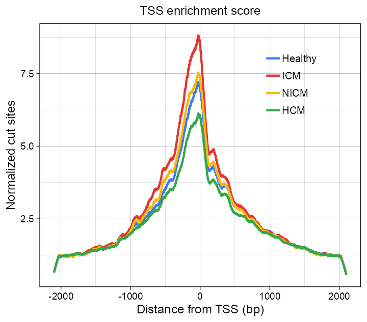
ggplot2::ggplot(
ggplot2::aes(
x = position,
y = score,
color = category
)
) +
ggplot2::geom_line(size = 0.5) +
ggplot2::scale_x_continuous(
name = "Distance from TSS (bp)",
breaks = c(101, 1101, 2101, 3101, 4100),
labels = seq(-2000, 2000, 1000)
) +
ggplot2::scale_y_continuous(
name = "Normalized cut sites"
) +
ggplot2::scale_color_manual(
name = NULL,
values = as.character(yarrr::piratepal(palette = "google"))
) +
ggplot2::ggtitle(label = "TSS enrichment score") +
ggplot2::theme_linedraw(base_size = 6, base_family = "Arial") +
ggplot2::theme(
legend.background = ggplot2::element_blank(),
legend.margin = ggplot2::margin(
t = 0, r = 0, b = 0, l = 0, unit = "mm"
),
legend.spacing.y = grid::unit(0, "mm"),
legend.key = ggplot2::element_blank(),
legend.key.size = grid::unit(3, "mm"),
legend.text = ggplot2::element_text(
family = "Arial",
size = 5,
margin = ggplot2::margin(
t = 0, r = 0, b = 0, l = -1, unit = "mm"
)
),
legend.position = c(0.7, 0.9),
legend.justification = c(0, 1),
plot.title = ggplot2::element_text(
family = "Arial", size = 6, hjust = 0.5
),
plot.background = ggplot2::element_blank()
)
List files.
fs::dir_ls(
path = file.path(
PROJECT_DIR,
"qc",
"tss_enrichment/raw/core_set_merged",
"cut_site"
),
regexp = "npy$"
)/Users/jialei/Dropbox/Data/Projects/UTSW/Cardiomyopathy/atac-seq/qc/tss_enrichment/raw/core_set_merged/cut_site/Aligned_sorted_deduped_q10_fresh_hcm_21_tss_flanking_0.npy
/Users/jialei/Dropbox/Data/Projects/UTSW/Cardiomyopathy/atac-seq/qc/tss_enrichment/raw/core_set_merged/cut_site/Aligned_sorted_deduped_q10_fresh_healthy_21_tss_flanking_0.npy
/Users/jialei/Dropbox/Data/Projects/UTSW/Cardiomyopathy/atac-seq/qc/tss_enrichment/raw/core_set_merged/cut_site/Aligned_sorted_deduped_q10_fresh_icm_21_tss_flanking_0.npy
/Users/jialei/Dropbox/Data/Projects/UTSW/Cardiomyopathy/atac-seq/qc/tss_enrichment/raw/core_set_merged/cut_site/Aligned_sorted_deduped_q10_fresh_nicm_21_tss_flanking_0.npyInspect data.
fs::dir_ls(
path = file.path(
PROJECT_DIR,
"qc",
"tss_enrichment/raw/core_set_merged",
"cut_site"
),
regexp = "npy$"
) |>
purrr::map(\(x) {
np$load(file = x) |>
{
\(y) {
y / mean(c(y[1:100], y[4102:4201]))
}
}() |>
tibble::enframe(name = "position", value = "score") |>
dplyr::mutate(
category = x |>
basename() |>
stringr::str_remove(
pattern = "Aligned_sorted_deduped_q10_"
) |>
stringr::str_remove(
pattern = "_21_tss_flanking_0.npy"
)
)
}) |>
dplyr::bind_rows() |>
dplyr::mutate(
category = category |> stringr::str_to_title(),
category = dplyr::case_when(
category == "Fresh_healthy" ~ "Healthy",
category == "Fresh_icm" ~ "ICM",
category == "Fresh_nicm" ~ "NICM",
category == "Fresh_hcm" ~ "HCM"
),
category = factor(
category,
levels = c("Healthy", "ICM", "NICM", "HCM")
)
) |>
head(n = 12)# A tibble: 12 × 3
position score category
<int> <dbl[1d]> <fct>
1 1 0.648 HCM
2 2 0.657 HCM
3 3 0.664 HCM
4 4 0.678 HCM
5 5 0.681 HCM
6 6 0.690 HCM
7 7 0.699 HCM
8 8 0.708 HCM
9 9 0.719 HCM
10 10 0.729 HCM
11 11 0.744 HCM
12 12 0.748 HCM dataset |>
dplyr::mutate(mt_ratio = num_reads_q10_mt / num_reads_q10) |>
dplyr::mutate(
category = factor(
category,
levels = c("Healthy", "ICM", "NICM", "HCM") |> rev()
)
) |>
ggplot2::ggplot(
ggplot2::aes(
x = mt_ratio, y = category, fill = category
)
) +
ggridges::geom_density_ridges(alpha = 0.8, color = NA) +
ggplot2::scale_x_continuous(
labels = scales::percent,
) +
ggplot2::scale_fill_manual(
values = yarrr::piratepal(palette = "google") |>
as.character() |> rev(),
) +
ggplot2::labs(x = "Mitochondrial read percentage", y = NULL) +
ggplot2::guides(fill = "none") +
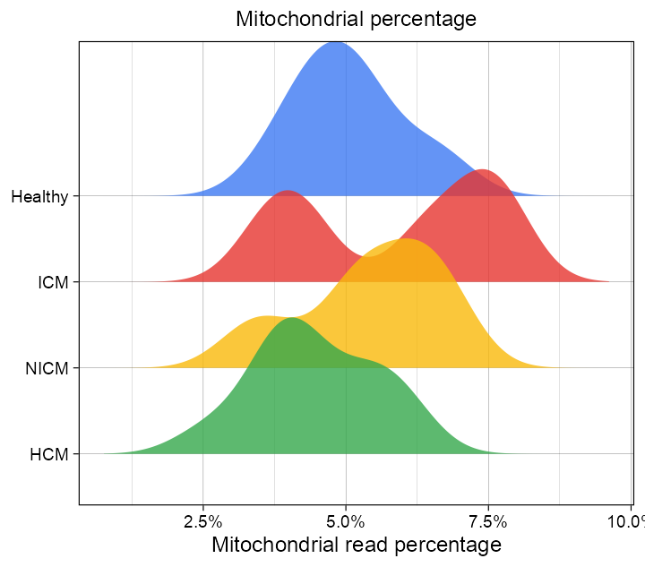
ggplot2::ggtitle(label = "Mitochondrial percentage") +
ggplot2::theme_linedraw(base_size = 6, base_family = "Arial") +
ggplot2::theme(
legend.background = ggplot2::element_blank(),
plot.title = ggplot2::element_text(
family = "Arial", size = 6, hjust = 0.5
),
plot.background = ggplot2::element_blank()
)
fs::dir_ls(
path = file.path(
PROJECT_DIR,
"qc",
"fragment_sizes",
"raw"
),
regexp = "fresh.+_CollectInsertSizeMetrics.txt"
) |>
purrr::map(\(x) {
readr::read_delim(
file = x,
delim = "\t",
skip = 11,
show_col_types = FALSE
) |>
normalize_fragment_sizes(
category = x |>
basename() |>
stringr::str_remove(
pattern = "_CollectInsertSizeMetrics.txt"
) |>
stringr::str_to_title()
)
}) |>
dplyr::bind_rows() |>
dplyr::mutate(
category = dplyr::case_when(
category == "Fresh_healthy" ~ "Healthy",
category == "Fresh_icm" ~ "ICM",
category == "Fresh_nicm" ~ "NICM",
category == "Fresh_hcm" ~ "HCM"
),
category = factor(
category,
levels = c(
"Healthy", "ICM", "NICM", "HCM"
)
)
) |>
ggplot2::ggplot(
ggplot2::aes(
x = insert_size,
y = norm_count,
color = category
)
) +
ggplot2::geom_line() +
ggplot2::scale_x_continuous(
name = "Fragment size (bp)",
limits = c(0, 1000),
breaks = seq(0, 1000, 200)
) +
ggplot2::scale_y_continuous(
name = "Norm. read density",
labels = scales::math_format(10^.x)
) +
ggplot2::annotation_logticks(base = 10, sides = "l", scaled = TRUE) +
ggplot2::scale_color_manual(
name = NULL,
values = as.character(yarrr::piratepal(palette = "google"))
) +
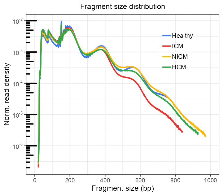
ggplot2::ggtitle(label = "Fragment size distribution") +
ggplot2::theme_bw(base_size = 6, base_family = "Arial") +
ggplot2::theme(
legend.background = ggplot2::element_blank(),
legend.margin = ggplot2::margin(
t = 0, r = 0, b = 0, l = 0, unit = "mm"
),
legend.spacing.y = ggplot2::unit(0, "mm"),
legend.key = ggplot2::element_blank(),
legend.key.size = ggplot2::unit(3, "mm"),
legend.text = ggplot2::element_text(
family = "Arial",
size = 5,
margin = ggplot2::margin(
t = 0, r = 0, b = 0, l = -1, unit = "mm"
)
),
legend.position = c(0.7, 0.9),
legend.justification = c(0, 1),
legend.box.background = ggplot2::element_blank(),
panel.background = ggplot2::element_blank(),
plot.title = ggplot2::element_text(
family = "Arial", size = 6, hjust = 0.5
),
plot.background = ggplot2::element_blank()
)
List files.
fs::dir_ls(
path = file.path(
PROJECT_DIR,
"qc",
"fragment_sizes",
"raw"
),
regexp = "fresh.+_CollectInsertSizeMetrics.txt"
)/Users/jialei/Dropbox/Data/Projects/UTSW/Cardiomyopathy/atac-seq/qc/fragment_sizes/raw/fresh_hcm_CollectInsertSizeMetrics.txt
/Users/jialei/Dropbox/Data/Projects/UTSW/Cardiomyopathy/atac-seq/qc/fragment_sizes/raw/fresh_healthy_CollectInsertSizeMetrics.txt
/Users/jialei/Dropbox/Data/Projects/UTSW/Cardiomyopathy/atac-seq/qc/fragment_sizes/raw/fresh_icm_CollectInsertSizeMetrics.txt
/Users/jialei/Dropbox/Data/Projects/UTSW/Cardiomyopathy/atac-seq/qc/fragment_sizes/raw/fresh_nicm_CollectInsertSizeMetrics.txtInspect data.
fs::dir_ls(
path = file.path(
PROJECT_DIR,
"qc",
"fragment_sizes",
"raw"
),
regexp = "fresh.+_CollectInsertSizeMetrics.txt"
) |>
purrr::map(\(x) {
readr::read_delim(
file = x,
delim = "\t",
skip = 11,
show_col_types = FALSE
) |>
normalize_fragment_sizes(
category = x |>
basename() |>
stringr::str_remove(
pattern = "_CollectInsertSizeMetrics.txt"
) |>
stringr::str_to_title()
)
}) |>
dplyr::bind_rows() |>
dplyr::mutate(
category = dplyr::case_when(
category == "Fresh_healthy" ~ "Healthy",
category == "Fresh_icm" ~ "ICM",
category == "Fresh_nicm" ~ "NICM",
category == "Fresh_hcm" ~ "HCM"
),
category = factor(
category,
levels = c(
"Healthy", "ICM", "NICM", "HCM"
)
)
) |>
head(n = 12)# A tibble: 12 × 6
insert_size All_Reads.fr_count All_Reads.rf_count all_reads_count norm_count
<dbl> <dbl> <dbl> <dbl> <dbl>
1 20 59 62 59 -6.53
2 21 81 100 81 -6.40
3 22 135 115 135 -6.17
4 23 169 174 169 -6.08
5 24 362 374 362 -5.75
6 25 1357 1427 1357 -5.17
7 26 23899 23859 23899 -3.93
8 27 49856 49877 49856 -3.61
9 28 46698 46688 46698 -3.64
10 29 46807 46847 46807 -3.63
11 30 42295 42213 42295 -3.68
12 31 36400 36158 36400 -3.74
# ℹ 1 more variable: category <fct>fragment_size <- fs::dir_ls(
path = file.path(
PROJECT_DIR,
"qc",
"fragment_sizes",
"raw"
),
regexp = "fresh.+_CollectInsertSizeMetrics.txt"
) |>
purrr::map(\(x) {
a <- readr::read_delim(
file = x,
delim = "\t",
skip = 11,
show_col_types = FALSE
)
a <- setNames(
object = a$All_Reads.fr_count,
nm = a$insert_size
)
a
})
names(fragment_size) <- names(fragment_size) |>
basename() |>
stringr::str_remove(
pattern = "_CollectInsertSizeMetrics.txt"
)z <- c("Healthy", "ICM", "NICM", "HCM")
purrr::map2(
c("fresh_healthy", "fresh_icm", "fresh_nicm", "fresh_hcm"), z, \(x, z) {
sample_name <- x
fragment_size_distribution <- fs::dir_ls(
path = file.path(
PROJECT_DIR,
"qc/chromatin_states",
"raw",
sample_name
),
regexp = "\\.txt"
) |>
purrr::map(\(y) {
sample_name <- stringr::str_remove(
string = basename(y),
pattern = ".+\\.bam_fragments_"
) |>
str_remove(
pattern = ".txt"
)
readr::read_delim(
file = file.path(
y
),
delim = "\t",
col_names = c("fragment_size", "count")
) |>
dplyr::filter(
fragment_size >= 50,
fragment_size <= 750
) |>
dplyr::mutate(
category = sample_name
) |>
dplyr::select(
fragment_size,
count,
category
)
})
fragment_size_distribution <- fragment_size_distribution |>
purrr::map(\(x) {
x[["percentage"]] <- (
x[["count"]] / (
fragment_size[[sample_name]]
)[x$fragment_size]
)
x[["value"]] <- as.vector(scale(x[["percentage"]]))
x_limits <- quantile(x[["value"]], c(0.1, 0.9))
x[["value"]][x[["value"]] <= x_limits[1]] <- x_limits[[1]]
x[["value"]][x[["value"]] >= x_limits[2]] <- x_limits[[2]]
x
})
fragment_size_distribution |>
dplyr::bind_rows() |>
dplyr::mutate(
category = factor(
category,
levels = c(
"CTCF_binding_site",
"promoter",
"promoter_flanking_region",
"enhancer",
"TF_binding_site",
"open_chromatin_region"
) |> rev()
)
) |>
ggplot2::ggplot(
ggplot2::aes(
x = fragment_size,
y = category,
fill = value
)
) +
ggplot2::geom_tile(ggplot2::aes(fill = value)) +
ggplot2::scale_fill_gradient2(name = NULL) +
ggplot2::scale_x_continuous(
name = "Fragment size (bp)",
limits = c(50, 750),
breaks = seq(50, 750, 175)
) +
ggplot2::scale_y_discrete(name = NULL) +
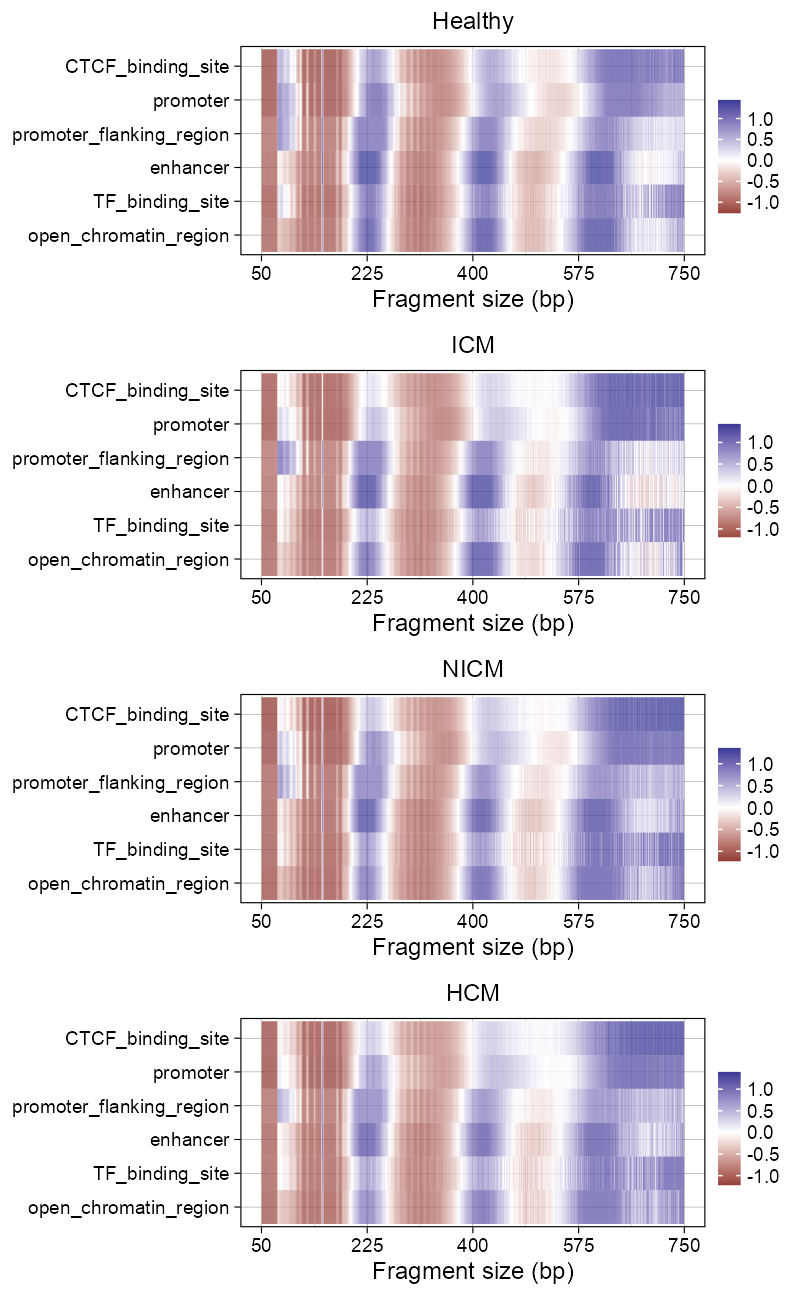
ggplot2::ggtitle(label = z) +
ggplot2::theme_linedraw(base_size = 6, base_family = "Arial") +
ggplot2::theme(
legend.background = ggplot2::element_blank(),
legend.margin = ggplot2::margin(
t = 0, r = 0, b = 0, l = 0, unit = "mm"
),
legend.key = ggplot2::element_blank(),
legend.key.height = ggplot2::unit(2, "mm"),
legend.key.width = ggplot2::unit(2, "mm"),
legend.text = ggplot2::element_text(
family = "Arial",
# size = 6,
margin = ggplot2::margin(
t = 0, r = 0, b = 0, l = -0.5, unit = "mm"
)
),
legend.box.margin = ggplot2::margin(
t = 0, r = 0, b = 0, l = -1, unit = "mm"
),
legend.box.background = ggplot2::element_blank(),
#
plot.title = ggplot2::element_text(
family = "Arial", size = 6, hjust = 0.5
)
)
}
) |>
purrr::reduce(`+`) +
patchwork::plot_layout(ncol = 1) +
patchwork::plot_annotation(
theme = ggplot2::theme(plot.margin = ggplot2::margin())
)
devtools::session_info()─ Session info ───────────────────────────────────────────────────────────────
setting value
version R version 4.3.1 (2023-06-16)
os macOS Ventura 13.5
system aarch64, darwin22.4.0
ui unknown
language (EN)
collate en_US.UTF-8
ctype en_US.UTF-8
tz America/Chicago
date 2023-08-12
pandoc 2.19.2 @ /Users/jialei/.pyenv/shims/ (via rmarkdown)
─ Packages ───────────────────────────────────────────────────────────────────
package * version date (UTC) lib source
BayesFactor 0.9.12-4.4 2022-07-05 [1] CRAN (R 4.3.0)
bit 4.0.5 2022-11-15 [1] CRAN (R 4.3.0)
bit64 4.0.5 2020-08-30 [1] CRAN (R 4.3.0)
cachem 1.0.8 2023-05-01 [1] CRAN (R 4.3.0)
callr 3.7.3 2022-11-02 [1] CRAN (R 4.3.0)
circlize 0.4.15 2022-05-10 [1] CRAN (R 4.3.0)
cli 3.6.1 2023-03-23 [1] CRAN (R 4.3.0)
coda 0.19-4 2020-09-30 [1] CRAN (R 4.3.0)
colorspace 2.1-0 2023-01-23 [1] CRAN (R 4.3.0)
crayon 1.5.2 2022-09-29 [1] CRAN (R 4.3.0)
devtools 2.4.5.9000 2023-08-11 [1] Github (r-lib/devtools@163c3f2)
digest 0.6.33 2023-07-07 [1] CRAN (R 4.3.1)
dplyr * 1.1.2.9000 2023-07-19 [1] Github (tidyverse/dplyr@c963d4d)
ellipsis 0.3.2 2021-04-29 [1] CRAN (R 4.3.0)
evaluate 0.21 2023-05-05 [1] CRAN (R 4.3.0)
extrafont * 0.19 2023-01-18 [1] CRAN (R 4.3.0)
extrafontdb 1.0 2012-06-11 [1] CRAN (R 4.3.0)
fansi 1.0.4 2023-01-22 [1] CRAN (R 4.3.0)
farver 2.1.1 2022-07-06 [1] CRAN (R 4.3.0)
fastmap 1.1.1 2023-02-24 [1] CRAN (R 4.3.0)
forcats * 1.0.0.9000 2023-04-23 [1] Github (tidyverse/forcats@4a8525a)
fs 1.6.3 2023-07-20 [1] CRAN (R 4.3.1)
generics 0.1.3 2022-07-05 [1] CRAN (R 4.3.0)
ggplot2 * 3.4.2.9000 2023-08-11 [1] Github (tidyverse/ggplot2@2cd0e96)
ggridges 0.5.5 2023-04-24 [1] Github (wilkelab/ggridges@543a092)
GlobalOptions 0.1.2 2020-06-10 [1] CRAN (R 4.3.0)
glue 1.6.2.9000 2023-04-23 [1] Github (tidyverse/glue@cbac82a)
gtable 0.3.3.9000 2023-04-23 [1] Github (r-lib/gtable@c56fd4f)
hms 1.1.3 2023-03-21 [1] CRAN (R 4.3.0)
htmltools 0.5.6 2023-08-10 [1] CRAN (R 4.3.1)
htmlwidgets 1.6.2 2023-03-17 [1] CRAN (R 4.3.0)
jpeg 0.1-10 2022-11-29 [1] CRAN (R 4.3.0)
jsonlite 1.8.7 2023-06-29 [1] CRAN (R 4.3.1)
knitr 1.43 2023-05-25 [1] CRAN (R 4.3.0)
labeling 0.4.2 2020-10-20 [1] CRAN (R 4.3.0)
lattice 0.21-8 2023-04-05 [2] CRAN (R 4.3.1)
lifecycle 1.0.3 2022-10-07 [1] CRAN (R 4.3.0)
lubridate * 1.9.2.9000 2023-07-22 [1] Github (tidyverse/lubridate@cae67ea)
magrittr 2.0.3 2022-03-30 [1] CRAN (R 4.3.0)
Matrix * 1.6-0 2023-07-08 [2] CRAN (R 4.3.1)
MatrixModels 0.5-2 2023-07-10 [1] CRAN (R 4.3.1)
memoise 2.0.1 2021-11-26 [1] CRAN (R 4.3.0)
munsell 0.5.0 2018-06-12 [1] CRAN (R 4.3.0)
mvtnorm 1.2-2 2023-06-08 [1] CRAN (R 4.3.0)
patchwork * 1.1.2.9000 2023-08-11 [1] Github (thomasp85/patchwork@bd57553)
pbapply 1.7-2 2023-06-27 [1] CRAN (R 4.3.1)
pillar 1.9.0 2023-03-22 [1] CRAN (R 4.3.0)
pkgbuild 1.4.2 2023-06-26 [1] CRAN (R 4.3.1)
pkgconfig 2.0.3 2019-09-22 [1] CRAN (R 4.3.0)
pkgload 1.3.2.9000 2023-07-05 [1] Github (r-lib/pkgload@3cf9896)
png 0.1-8 2022-11-29 [1] CRAN (R 4.3.0)
prettyunits 1.1.1.9000 2023-04-23 [1] Github (r-lib/prettyunits@8706d89)
processx 3.8.2 2023-06-30 [1] CRAN (R 4.3.1)
ps 1.7.5 2023-04-18 [1] CRAN (R 4.3.0)
purrr * 1.0.2.9000 2023-08-11 [1] Github (tidyverse/purrr@ac4f5a9)
R.cache 0.16.0 2022-07-21 [1] CRAN (R 4.3.0)
R.methodsS3 1.8.2 2022-06-13 [1] CRAN (R 4.3.0)
R.oo 1.25.0 2022-06-12 [1] CRAN (R 4.3.0)
R.utils 2.12.2 2022-11-11 [1] CRAN (R 4.3.0)
R6 2.5.1.9000 2023-04-23 [1] Github (r-lib/R6@e97cca7)
ragg 1.2.5 2023-01-12 [1] CRAN (R 4.3.0)
Rcpp 1.0.11 2023-07-06 [1] CRAN (R 4.3.1)
readr * 2.1.4.9000 2023-08-03 [1] Github (tidyverse/readr@80e4dc1)
remotes 2.4.2.9000 2023-06-09 [1] Github (r-lib/remotes@8875171)
reticulate 1.31 2023-08-10 [1] CRAN (R 4.3.1)
rlang 1.1.1.9000 2023-06-09 [1] Github (r-lib/rlang@c55f602)
rmarkdown 2.23.4 2023-07-27 [1] Github (rstudio/rmarkdown@054d735)
rstudioapi 0.15.0.9000 2023-07-19 [1] Github (rstudio/rstudioapi@feceaef)
Rttf2pt1 1.3.12 2023-01-22 [1] CRAN (R 4.3.0)
scales 1.2.1 2022-08-20 [1] CRAN (R 4.3.0)
sessioninfo 1.2.2 2021-12-06 [1] CRAN (R 4.3.0)
shape 1.4.6 2021-05-19 [1] CRAN (R 4.3.0)
stringi 1.7.12 2023-01-11 [1] CRAN (R 4.3.0)
stringr * 1.5.0.9000 2023-08-11 [1] Github (tidyverse/stringr@08ff36f)
styler * 1.10.1 2023-07-17 [1] Github (r-lib/styler@aca7223)
systemfonts 1.0.4 2022-02-11 [1] CRAN (R 4.3.0)
textshaping 0.3.6 2021-10-13 [1] CRAN (R 4.3.0)
tibble * 3.2.1.9005 2023-05-28 [1] Github (tidyverse/tibble@4de5c15)
tidyr * 1.3.0.9000 2023-04-23 [1] Github (tidyverse/tidyr@0764e65)
tidyselect 1.2.0 2022-10-10 [1] CRAN (R 4.3.0)
tidyverse * 2.0.0.9000 2023-04-23 [1] Github (tidyverse/tidyverse@8ec2e1f)
timechange 0.2.0 2023-01-11 [1] CRAN (R 4.3.0)
tzdb 0.4.0 2023-05-12 [1] CRAN (R 4.3.0)
usethis 2.2.2.9000 2023-07-11 [1] Github (r-lib/usethis@467ff57)
utf8 1.2.3 2023-01-31 [1] CRAN (R 4.3.0)
vctrs 0.6.3 2023-06-14 [1] CRAN (R 4.3.0)
vroom 1.6.3.9000 2023-04-30 [1] Github (tidyverse/vroom@89b6aac)
withr 2.5.0 2022-03-03 [1] CRAN (R 4.3.0)
xfun 0.40 2023-08-09 [1] CRAN (R 4.3.1)
yaml 2.3.7 2023-01-23 [1] CRAN (R 4.3.0)
yarrr 0.1.6 2023-04-23 [1] Github (ndphillips/yarrr@e2e4488)
[1] /opt/homebrew/lib/R/4.3/site-library
[2] /opt/homebrew/Cellar/r/4.3.1/lib/R/library
─ Python configuration ───────────────────────────────────────────────────────
python:         /Users/jialei/.pyenv/shims/python
libpython:      /Users/jialei/.pyenv/versions/mambaforge-22.9.0-3/lib/libpython3.10.dylib
pythonhome:     /Users/jialei/.pyenv/versions/mambaforge-22.9.0-3:/Users/jialei/.pyenv/versions/mambaforge-22.9.0-3
version:        3.10.9 | packaged by conda-forge | (main, Feb  2 2023, 20:26:08) [Clang 14.0.6 ]
numpy:          /Users/jialei/.pyenv/versions/mambaforge-22.9.0-3/lib/python3.10/site-packages/numpy
numpy_version:  1.24.3
numpy:          /Users/jialei/.pyenv/versions/mambaforge-22.9.0-3/lib/python3.10/site-packages/numpy

NOTE: Python version was forced by RETICULATE_PYTHON
──────────────────────────────────────────────────────────────────────────────@article{bhattacharyya2023,
author = {Bhattacharyya, Samadrita and Duan, Jialei and J. Vela, Ryan
and Bhakta, Minoti and Bajona, Pietro and P.A. Mammen, Pradeep and
C. Hon, Gary and V. Munshi, Nikhil},
publisher = {American Heart Association},
title = {Accurate {Classification} of {Cardiomyopathy} {Diagnosis} by
{Chromatin} {Accessibility}},
journal = {Circulation},
volume = {146},
number = {11},
pages = {878 - 881},
date = {2023-08-12},
url = {https://doi.org/10.1161/CIRCULATIONAHA.122.059659},
doi = {10.1161/CIRCULATIONAHA.122.059659},
langid = {en}
}