
Sys.time()[1] "2023-08-12 00:21:49 CDT"Reprogram-Seq leverages organ-specific cell atlas data with single-cell perturbation and computational analysis to predict, evaluate, and optimize TF combinations that reprogram a cell type of interest.
Sys.time()[1] "2023-08-12 00:21:49 CDT"[1] "America/Chicago"Load required packages.
`%+replace%` <- ggplot2::`%+replace%`PROJECT_DIR <- file.path(
"/Users/jialei/Dropbox/Data/Projects/UTSW/Cellular_reprogramming",
"Cardiac_reprogramming/Notebooks"
)gene_symbols <- vroom::vroom(
file = file.path(
PROJECT_DIR, "data", "misc", "genes.tsv"
),
col_names = FALSE
)
gene_symbols <- setNames(object = gene_symbols$X2, nm = gene_symbols$X1)
gene_symbols |> head()ENSMUSG00000051951 ENSMUSG00000089699 ENSMUSG00000102343 ENSMUSG00000025900
"Xkr4" "Gm1992" "Gm37381" "Rp1"
ENSMUSG00000109048 ENSMUSG00000025902
"Rp1" "Sox17" length(gene_symbols)[1] 27999matrix_readcount_use <- Matrix::sparseMatrix(
i = readRDS(
file.path(
PROJECT_DIR, "data/drop-seq", "expr_readcount_raw_csc_indices.rds"
)
),
p = readRDS(
file.path(
PROJECT_DIR, "data/drop-seq", "expr_readcount_raw_csc_indptr.rds"
)
),
x = readRDS(
file.path(
PROJECT_DIR, "data/drop-seq", "expr_readcount_raw_csc_values.rds"
)
),
dims = readRDS(
file.path(
PROJECT_DIR, "data/drop-seq", "expr_readcount_raw_csc_shape.rds"
)
),
dimnames = readRDS(
file.path(
PROJECT_DIR, "data/drop-seq", "expr_readcount_raw_csc_dimnames.rds"
)
),
index1 = FALSE
)dim(matrix_readcount_use)[1] 27999 27416rownames(matrix_readcount_use) <- paste(
rownames(matrix_readcount_use),
gene_symbols[rownames(matrix_readcount_use)],
sep = "_"
)
matrix_readcount_use[1:5, 1:5] |>
as.matrix() |>
knitr::kable()| JD126-1-2_TTTCTATATACA.bam | JD126-1-2_CCTAGAAACCAG.bam | JD126-1-2_TCATAGTCTATT.bam | JD126-1-2_ATGACCTTTCCC.bam | JD126-1-2_CATTAGTGATGG.bam | |
|---|---|---|---|---|---|
| ENSMUSG00000051951_Xkr4 | 0 | 0 | 0 | 0 | 0 |
| ENSMUSG00000089699_Gm1992 | 0 | 0 | 0 | 0 | 0 |
| ENSMUSG00000102343_Gm37381 | 0 | 0 | 0 | 0 | 0 |
| ENSMUSG00000025900_Rp1 | 0 | 0 | 0 | 0 | 0 |
| ENSMUSG00000109048_Rp1 | 0 | 0 | 0 | 0 | 0 |
dim(embedding)[1] 25776 7Check memory usage.
purrr::walk(
    list(matrix_readcount_use, embedding), \(x) {
        print(object.size(x), units = "auto", standard = "SI")
    }
)
751.2 MB
3.4 MBx_column <- "x"
y_column <- "y"
GEOM_POINT_SIZE <- 0.5
EMBEDDING_TITLE_PREFIX <- "t-SNE"
RASTERISED <- FALSEembedding |>
tibble::rownames_to_column(var = "cell") |>
dplyr::mutate(
num_umis = colSums(matrix_readcount_use[, cell]),
num_features = colSums(matrix_readcount_use[, cell] > 0),
) |>
dplyr::rename(batch = batch.id) |>
dplyr::group_by(batch) |>
dplyr::summarise(
num_cells = n(),
median_umis = median(num_umis),
median_features = median(num_features)
) |>
gt::gt() |>
gt::data_color(
columns = c(median_umis),
fn = scales::col_numeric(
palette = c(
"green", "orange", "red"
),
domain = NULL
)
) |>
gt::fmt_number(
columns = c(num_cells),
sep_mark = ",",
decimals = 0
) |>
gt::fmt_number(
columns = c(median_umis, median_features),
sep_mark = ",",
decimals = 1
) |>
gt::grand_summary_rows(
columns = c(batch),
fns = list(
Count = ~ n()
),
fmt = ~ gt::fmt_number(., decimals = 0, use_seps = TRUE)
) |>
gt::grand_summary_rows(
columns = c(num_cells:median_features),
fns = list(
Mean = ~ mean(.)
),
fmt = ~ gt::fmt_number(., decimals = 1, use_seps = TRUE)
) |>
gt::grand_summary_rows(
columns = c(num_cells),
fns = list(
Sum = ~ sum(.)
),
fmt = ~ gt::fmt_number(., decimals = 0, use_seps = TRUE)
) |>
gt::tab_header(
title = gt::md("**Drop-Seq**; Batch")
) |>
gt::tab_source_note(
source_note = gt::md(
"***[Here](https://www.ncbi.nlm.nih.gov/geo/query/acc.cgi?acc=GSE117795)** are the details.*"
)
)| Drop-Seq; Batch | ||||
| batch | num_cells | median_umis | median_features | |
|---|---|---|---|---|
| JD126-1-2 | 335 | 3,697.0 | 1,839.0 | |
| JD126A1 | 289 | 3,499.0 | 1,669.0 | |
| JD126A5 | 310 | 3,575.0 | 1,759.5 | |
| JD126B | 625 | 3,604.0 | 1,733.0 | |
| JD131-A | 418 | 1,765.0 | 1,105.0 | |
| JD131-B | 371 | 1,895.0 | 1,146.0 | |
| JD131-C | 381 | 1,894.0 | 1,168.0 | |
| JD135A | 101 | 3,203.0 | 1,521.0 | |
| JD135Y | 222 | 1,755.5 | 1,007.0 | |
| JD135Z | 92 | 1,890.0 | 966.5 | |
| JD136A | 172 | 2,348.5 | 1,285.5 | |
| JD136B | 269 | 1,603.0 | 975.0 | |
| JD136C | 168 | 1,140.5 | 734.0 | |
| JD136DE | 370 | 1,042.5 | 694.0 | |
| JD136F | 251 | 1,752.0 | 993.0 | |
| JD136G | 500 | 1,341.5 | 827.0 | |
| JD137A | 268 | 2,796.5 | 1,410.5 | |
| JD145A1 | 269 | 3,332.0 | 1,623.0 | |
| JD145A5 | 267 | 2,911.0 | 1,503.0 | |
| JD145B1 | 284 | 3,531.5 | 1,704.0 | |
| JD145B5 | 287 | 1,905.0 | 1,045.0 | |
| JD145C | 169 | 2,235.0 | 1,056.0 | |
| JD145D | 187 | 1,797.0 | 941.0 | |
| JD145E | 287 | 977.0 | 590.0 | |
| JD145F | 103 | 533.0 | 396.0 | |
| JD146A1 | 530 | 3,210.5 | 1,555.5 | |
| JD146A5 | 549 | 4,260.0 | 1,935.0 | |
| JD146B1 | 466 | 4,879.5 | 1,973.0 | |
| JD146B5 | 444 | 4,035.5 | 1,828.0 | |
| JD146C1 | 452 | 5,129.5 | 2,004.5 | |
| JD146C5 | 420 | 2,922.0 | 1,399.5 | |
| JD149A | 275 | 1,118.0 | 699.0 | |
| JD149B | 251 | 823.0 | 531.0 | |
| JD149C | 382 | 1,179.5 | 747.5 | |
| JD149D | 365 | 1,054.0 | 688.0 | |
| JD149E | 236 | 854.5 | 603.0 | |
| JD150-3A | 393 | 1,486.0 | 911.0 | |
| JD150-3B | 345 | 1,624.0 | 1,002.0 | |
| JD150-3C | 487 | 2,110.0 | 1,190.0 | |
| JD150-4A | 330 | 1,652.0 | 962.0 | |
| JD150-4B | 370 | 1,476.5 | 893.5 | |
| JD150A | 342 | 778.5 | 487.0 | |
| JD150B | 317 | 849.0 | 564.0 | |
| JD150C | 346 | 1,372.0 | 888.5 | |
| JD150D | 465 | 1,081.0 | 723.0 | |
| JD164_165 | 272 | 3,324.5 | 1,935.5 | |
| JD166_167 | 204 | 6,267.5 | 3,047.0 | |
| JD168A | 252 | 11,674.5 | 4,225.0 | |
| JD168B | 240 | 4,899.5 | 2,510.5 | |
| JD168C | 182 | 14,665.5 | 4,678.5 | |
| JD168_169 | 236 | 4,234.5 | 2,302.5 | |
| JD169A | 306 | 7,700.0 | 3,450.0 | |
| JD169B | 178 | 13,284.5 | 4,515.5 | |
| JD169C | 206 | 10,929.5 | 4,092.0 | |
| JD170A | 148 | 11,175.0 | 4,197.0 | |
| JD170B | 108 | 12,311.0 | 4,191.0 | |
| JD170C | 150 | 11,961.5 | 4,228.0 | |
| JD170_171 | 288 | 13,620.5 | 4,505.5 | |
| JD171A | 270 | 7,281.0 | 3,207.0 | |
| JD171B | 224 | 11,545.0 | 4,211.5 | |
| JD171C | 166 | 9,291.0 | 3,673.0 | |
| PZ473 | 168 | 9,368.5 | 3,888.5 | |
| PZ474 | 188 | 6,470.0 | 3,116.5 | |
| PZ475 | 326 | 11,516.5 | 4,077.0 | |
| PZ476 | 292 | 10,177.5 | 3,943.0 | |
| PZ477 | 552 | 5,562.5 | 2,731.0 | |
| PZ478 | 344 | 7,171.0 | 3,283.5 | |
| PZ479 | 356 | 9,106.0 | 3,655.0 | |
| PZ480 | 196 | 10,180.5 | 3,878.5 | |
| PZ481 | 132 | 11,876.5 | 4,161.0 | |
| PZ482 | 70 | 4,286.0 | 2,213.0 | |
| PZ483 | 98 | 4,452.5 | 2,233.5 | |
| PZ484 | 224 | 9,902.5 | 3,863.5 | |
| PZ485 | 264 | 10,482.5 | 3,963.5 | |
| PZ486 | 344 | 6,220.0 | 2,901.5 | |
| PZ487 | 238 | 5,281.5 | 2,571.5 | |
| PZ492 | 399 | 1,618.0 | 960.0 | |
| PZ493 | 241 | 1,394.0 | 841.0 | |
| PZ496 | 344 | 7,004.5 | 3,245.0 | |
| PZ497 | 208 | 9,547.0 | 3,810.5 | |
| PZ580 | 472 | 8,199.5 | 3,482.5 | |
| PZ581 | 360 | 6,468.0 | 3,058.5 | |
| PZ582 | 214 | 9,730.5 | 3,892.5 | |
| PZ583 | 120 | 10,060.5 | 3,977.0 | |
| PZ584 | 190 | 14,141.5 | 4,915.0 | |
| PZ585 | 152 | 15,586.5 | 4,924.0 | |
| PZ586 | 292 | 4,879.0 | 2,466.5 | |
| PZ587 | 204 | 11,968.5 | 4,318.5 | |
| PZ588 | 110 | 24,547.5 | 5,941.0 | |
| PZ589 | 110 | 11,439.0 | 3,965.5 | |
| PZ590 | 94 | 17,243.5 | 5,124.5 | |
| PZ660 | 148 | 2,893.5 | 1,478.0 | |
| PZ661 | 136 | 2,414.5 | 1,289.5 | |
| Count | 93 | — | — | — |
| Mean | — | 277.2 | 5,734.1 | 2,348.6 |
| Sum | — | 25,776 | — | — |
| Here are the details. | ||||
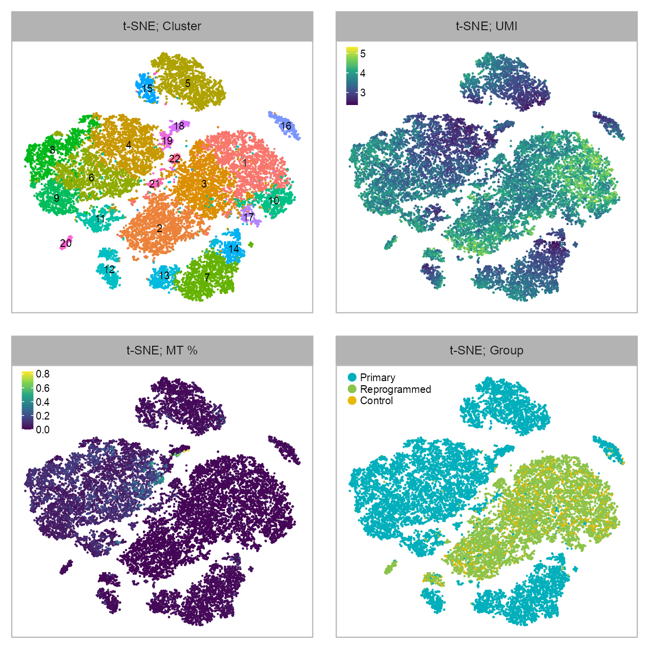
p_embedding_cluster <- plot_embedding(
    data = embedding[, c(x_column, y_column)],
    color = embedding$cluster |> as.factor(),
    label = glue::glue("{EMBEDDING_TITLE_PREFIX}; Cluster"),
    color_labels = TRUE,
    color_legend = FALSE,
    sort_values = FALSE,
    rasterise = RASTERISED,
    geom_point_size = GEOM_POINT_SIZE
) +
    theme_customized_embedding()

p_embedding_UMI <- plot_embedding(
    data = embedding[, c(x_column, y_column)],
    color = log10(Matrix::colSums(matrix_readcount_use[, embedding$cell])),
    label = glue::glue("{EMBEDDING_TITLE_PREFIX}; UMI"),
    color_legend = TRUE,
    sort_values = FALSE,
    shuffle_values = TRUE,
    rasterise = RASTERISED,
    geom_point_size = GEOM_POINT_SIZE
) +
    theme_customized_embedding()

p_embedding_MT <- plot_embedding(
    data = embedding[, c(x_column, y_column)],
    color = (colSums(matrix_readcount_use[
        stringr::str_detect(
            string = stringr::str_remove(
                string = rownames(matrix_readcount_use),
                pattern = "^E.+_"
            ),
            pattern = "mt-"
        ),
    ]) / colSums(matrix_readcount_use))[embedding$cell],
    label = glue::glue("{EMBEDDING_TITLE_PREFIX}; MT %"),
    color_legend = TRUE,
    sort_values = TRUE,
    shuffle_values = FALSE,
    rasterise = RASTERISED,
    geom_point_size = GEOM_POINT_SIZE
) + theme_customized_embedding()

p_embedding_group <- plot_embedding(
    data = embedding[, c(x_column, y_column)],
    color = embedding$group |> as.factor(),
    label = glue::glue("{EMBEDDING_TITLE_PREFIX}; Group"),
    color_labels = FALSE,
    color_legend = TRUE,
    sort_values = FALSE,
    shuffle_values = TRUE,
    rasterise = RASTERISED,
    geom_point_size = GEOM_POINT_SIZE
) +
    theme_customized_embedding() +
    ggplot2::scale_color_manual(
        values = c(
            Primary = "#00AFBB",
            Reprogrammed = "#8BC34A",
            Control = "#E7B800"
        )
    )
embedding |>
dplyr::mutate(
num_umis = colSums(matrix_readcount_use[, cell]),
num_features = colSums(matrix_readcount_use[, cell] > 0),
) |>
dplyr::group_by(cluster) |>
dplyr::summarise(
num_cells = n(),
median_umis = median(num_umis),
median_features = median(num_features)
) |>
gt::gt() |>
gt::data_color(
columns = c(median_umis),
fn = scales::col_numeric(
palette = c(
"green", "orange", "red"
),
domain = NULL
)
) |>
gt::fmt_number(
columns = c(num_cells),
sep_mark = ",",
decimals = 0
) |>
gt::fmt_number(
columns = c(median_umis, median_features),
sep_mark = ",",
decimals = 1
) |>
gt::grand_summary_rows(
columns = c(cluster),
fns = list(
Count = ~ n()
),
fmt = ~ gt::fmt_number(., decimals = 0, use_seps = TRUE)
) |>
gt::grand_summary_rows(
columns = c(median_umis:median_features),
fns = list(
Mean = ~ mean(.)
),
fmt = ~ gt::fmt_number(., decimals = 1, use_seps = TRUE)
) |>
gt::grand_summary_rows(
columns = c(num_cells),
fns = list(
Sum = ~ sum(.)
),
fmt = ~ gt::fmt_number(., decimals = 0, use_seps = TRUE)
) |>
gt::tab_header(
title = gt::md("**Drop-Seq**; Clustering")
)| Drop-Seq; Clustering | ||||
| cluster | num_cells | median_umis | median_features | |
|---|---|---|---|---|
| 1 | 2,875 | 13,196.0 | 4,578.0 | |
| 2 | 2,798 | 8,594.0 | 3,639.5 | |
| 3 | 2,786 | 6,165.0 | 2,905.0 | |
| 4 | 2,710 | 933.0 | 561.5 | |
| 5 | 2,356 | 1,505.5 | 1,013.0 | |
| 6 | 2,139 | 2,590.0 | 1,249.0 | |
| 7 | 1,934 | 2,238.5 | 1,347.0 | |
| 8 | 1,575 | 5,225.0 | 1,891.0 | |
| 9 | 1,075 | 5,719.0 | 2,203.0 | |
| 10 | 871 | 12,955.0 | 4,294.0 | |
| 11 | 708 | 4,111.0 | 1,872.5 | |
| 12 | 681 | 3,495.0 | 1,956.0 | |
| 13 | 669 | 2,438.0 | 1,483.0 | |
| 14 | 556 | 725.0 | 530.5 | |
| 15 | 478 | 2,661.0 | 1,606.5 | |
| 16 | 474 | 1,368.0 | 906.5 | |
| 17 | 254 | 4,995.5 | 2,172.5 | |
| 18 | 236 | 1,737.0 | 256.5 | |
| 19 | 181 | 620.0 | 372.0 | |
| 20 | 165 | 9,490.0 | 3,679.0 | |
| 21 | 133 | 5,234.0 | 2,464.0 | |
| 22 | 122 | 6,274.0 | 2,877.0 | |
| Count | 22 | — | — | — |
| Mean | — | — | 4,648.6 | 1,993.5 |
| Sum | — | 25,776 | — | — |
purrr::reduce(
    list(
        p_embedding_cluster,
        p_embedding_UMI,
        p_embedding_MT,
        p_embedding_group
    ),
    `+`
) +
    patchwork::plot_layout(ncol = 2) +
    patchwork::plot_annotation(
        theme = ggplot2::theme(plot.margin = ggplot2::margin())
    )
Attaching package: 'formattable'The following object is masked from 'package:patchwork':
areaembedding |>
dplyr::mutate(
num_umis = colSums(matrix_readcount_use[, cell]),
num_features = colSums(matrix_readcount_use[, cell] > 0),
) |>
dplyr::group_by(group) |>
dplyr::summarise(
num_cells = n(),
median_umis = median(num_umis),
median_features = median(num_features)
) |>
formattable::formattable(
list(
# num_cells = formattable::color_tile("transparent", "lightpink"),
num_cells = formattable::color_bar("Lightpink"),
median_umis = formattable::color_bar("lightgreen"),
median_features = formattable::color_bar("lightblue")
),
full_width = FALSE,
caption = "Drop-Seq; Group"
)| group | num_cells | median_umis | median_features |
|---|---|---|---|
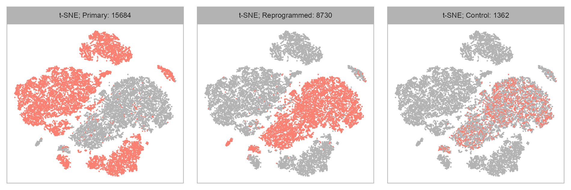
| Primary | 15684 | 2030 | 1139 |
| Reprogrammed | 8730 | 8532 | 3562 |
| Control | 1362 | 9383 | 3789 |
purrr::map(levels(embedding$group), \(x) {
    plot_embedding(
        data = embedding[, c(x_column, y_column)],
        color = as.integer(embedding$group == x) |> as.factor(),
        label = glue::glue(
            "{EMBEDDING_TITLE_PREFIX}; {x}: {sum(embedding$group == x)}"
        ),
        color_labels = FALSE,
        color_legend = FALSE,
        sort_values = TRUE,
        shuffle_values = FALSE,
        rasterise = RASTERISED,
        geom_point_size = GEOM_POINT_SIZE
    ) +
        theme_customized_embedding() +
        ggplot2::scale_color_manual(
            values = c("grey70", "salmon")
        )
}) |>
    purrr::reduce(`+`) +
    patchwork::plot_layout(ncol = 3) +
    patchwork::plot_annotation(
        theme = ggplot2::theme(plot.margin = ggplot2::margin())
    )
Extract colors from the initial plots to keep colors consistent.
color_palette <- ggplot2::ggplot_build(p_embedding_cluster)$data[[1]] |>
    dplyr::select(color = colour, cluster = group) |>
    unique() |>
    dplyr::arrange(cluster)

color_palette <- setNames(
    object = color_palette$color,
    nm = color_palette$cluster
)

scales::show_col(color_palette, borders = NA)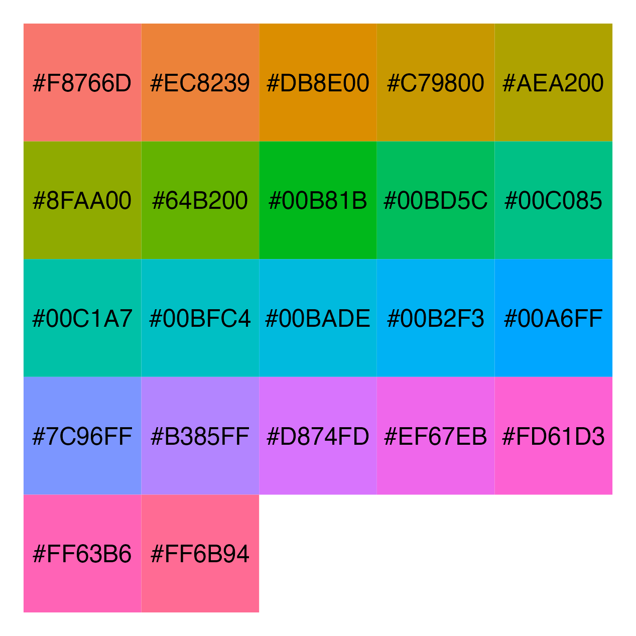
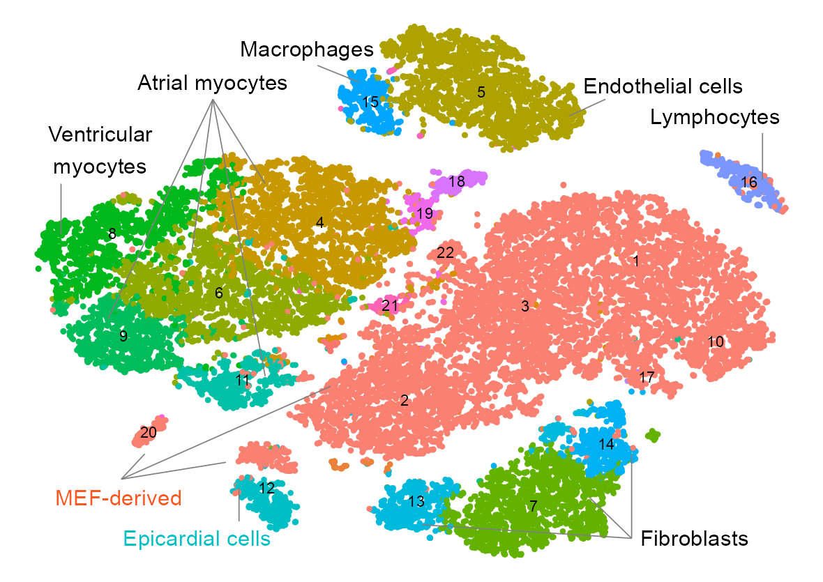
cell_type_segments <- data.frame(
    x = c(
        -40, -40, -40, -40, -69, -35, 40, 40, 40, 65, 28, -12, -57.5,
        -57.5, -57.5
    ),
    y = c(
        60, 60, 60, 60, 20, -55, -70, -70, -70, 50, 55, 65, -52.5,
        -52.5, -52.5
    ),
    xend = c(
        -30, -44, -60, -30, -69, -35, 32, 0, 40, 65, 35, -20, -17.5,
        -53, -37.5
    ),
    yend = c(
        35, 15, -5, -22, 35, -65, -58, -66, -45, 36, 60, 70, -25,
        -45, -47.5
    ),
    cluster = c(4, 6, 9, 11, 8, 12, 7, 13, 14, 16, 5, 15, 2, 20, 12)
)

cell_type_labels <- data.frame(
    x = c(-40, -61.5, -43, 52, 56, 46, -22, -58),
    y = c(65, 45, -70, -70, 55, 64, 75, -58),
    label = c(
        "Atrial myocytes",
        "Ventricular\nmyocytes",
        "Epicardial cells",
        "Fibroblasts",
        "Lymphocytes",
        "Endothelial cells",
        "Macrophages",
        "MEF-derived"
    )
)

cluster_labels <- embedding |>
    dplyr::group_by(cluster) |>
    dplyr::summarise(
        x = median(x),
        y = median(y)
    ) |>
    as.data.frame()

plot_embedding(
    data = embedding[, c(x_column, y_column)],
    color = embedding |>
        dplyr::mutate(
            color_group = dplyr::case_when(
                group %in% c("Reprogrammed", "Control") ~ "MEF-derived",
                TRUE ~ as.character(cluster)
            )
        ) |>
        dplyr::pull(color_group) |> as.factor(),
    label = NULL,
    color_labels = FALSE,
    color_legend = FALSE,
    sort_values = FALSE,
    rasterise = RASTERISED,
    geom_point_size = GEOM_POINT_SIZE * 2
) +
    theme_customized_embedding(void = TRUE) +
    ggplot2::scale_color_manual(
        values = c(color_palette, "MEF-derived" = "salmon")
    ) +
    ggplot2::geom_segment(
        data = cell_type_segments,
        ggplot2::aes(x = x, xend = xend, y = y, yend = yend),
        color = "grey50",
        size = .2
    ) +
    ggplot2::geom_text(
        data = cell_type_labels,
        ggplot2::aes(x, y, label = label),
        color = c(rep("black", 2), "#00BFC4", rep("black", 4), "#FF5722"),
        size = 2.8,
        family = "Arial"
    ) +
    ggplot2::annotate(
        geom = "text",
        family = "Arial",
        x = cluster_labels[, "x"],
        y = cluster_labels[, "y"], label = cluster_labels[, 1],
        parse = TRUE,
        size = 2,
        color = c("black")
    )
pdf_width <- 104
pdf_height <- 74
file_name <- glue::glue(
    "Rplot_embedding_dropseq_{EMBEDDING_TITLE_PREFIX}_",
    "cell_group_{pdf_width}_{pdf_height}.pdf"
)
if (!file.exists(file_name)) {
    ggplot2::ggsave(
        filename = file_name,
        useDingbats = FALSE,
        plot = ggplot2::last_plot(),
        device = NULL,
        path = NULL,
        scale = 1,
        width = pdf_width,
        height = pdf_height,
        units = c("mm"),
    )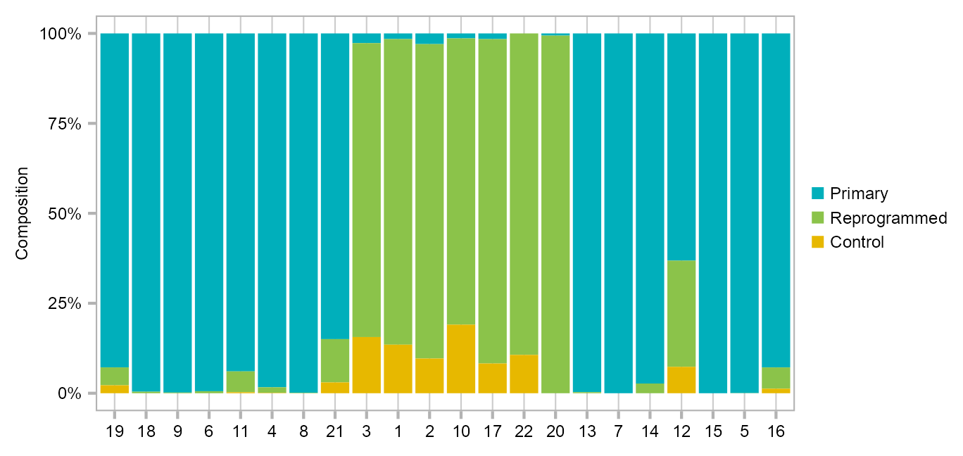
}Bar charts indicating the cellar composition of t-SNE clusters defined in Figure 1B.
calc_group_composition(
    data = embedding,
    x = "cluster",
    group = "group"
) |>
    dplyr::mutate(
        cluster = factor(
            cluster,
            levels = c(
                19, 18,
                9, 6, 11, 4, 8, 21,
                3, 1, 2, 10, 17, 22, 20,
                13, 7, 14, 12, 15, 5, 16
            )
        )
    ) |>
    plot_barplot(
        x = "cluster",
        y = "percentage",
        z = "group",
        legend_ncol = 1
    ) +
    ggplot2::scale_fill_manual(
        values = c(
            Primary = "#00AFBB",
            Reprogrammed = "#8BC34A",
            Control = "#E7B800"
        )
    )
FEATURES_SELECTED <- c(
    "ENSMUSG00000009471_Myod1",
    "ENSMUSG00000026414_Tnnt2",
    "ENSMUSG00000016458_Wt1",
    "ENSMUSG00000025105_Bnc1",
    "ENSMUSG00000049382_Krt8",
    "ENSMUSG00000079018_Ly6c1",
    "ENSMUSG00000049436_Upk1b",
    "ENSMUSG00000021391_Cenpp"
)purrr::map(FEATURES_SELECTED, \(x) {
selected_feature <- x
cat(selected_feature, "\n")
values <- log10(
calc_cpm(matrix_readcount_use[, embedding$cell])
[selected_feature, ] + 1
)
p1 <- plot_embedding(
data = embedding[, c(x_column, y_column)],
color = values,
label = paste(
EMBEDDING_TITLE_PREFIX,
selected_feature |> stringr::str_remove(pattern = "^E.+_"),
sep = "; "
),
color_legend = TRUE,
sort_values = TRUE,
rasterise = RASTERISED,
geom_point_size = GEOM_POINT_SIZE * 1.25,
na_value = "grey80"
) +
theme_customized_embedding()
return(p1)
}) |>
# unlist(recursive = FALSE) |>
purrr::reduce(`+`) +
patchwork::plot_layout(ncol = 2, byrow = FALSE) +
patchwork::plot_annotation(
theme = ggplot2::theme(plot.margin = ggplot2::margin())
)ENSMUSG00000009471_Myod1
ENSMUSG00000026414_Tnnt2
ENSMUSG00000016458_Wt1
ENSMUSG00000025105_Bnc1
ENSMUSG00000049382_Krt8
ENSMUSG00000079018_Ly6c1
ENSMUSG00000049436_Upk1b
ENSMUSG00000021391_Cenpp 
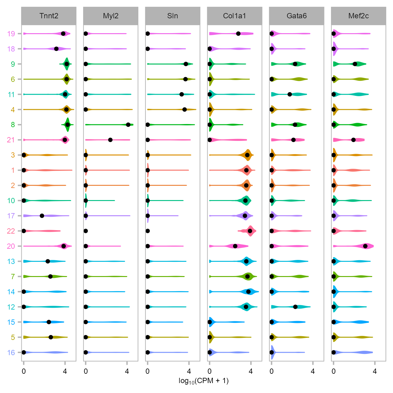
Violin plot illustrating the expression of cardiac markers from single-cell expression data derived from P0 mouse heart and reprogrammed/uninfected MEFs.
labels_y <- c(
    19, 18,
    9, 6, 11, 4, 8, 21,
    3, 1, 2, 10, 17, 22, 20,
    13, 7, 14, 12, 15, 5, 16
)

plot_violin(
    cells = embedding |>
        dplyr::mutate(
            cluster = factor(
                cluster,
                levels = labels_y
            )
        ) |>
        split(~cluster) |>
        purrr::map(\(x) {
            x |> dplyr::pull(cell)
        }),
    features = c(
        "ENSMUSG00000026414_Tnnt2",
        "ENSMUSG00000013936_Myl2",
        "ENSMUSG00000042045_Sln",
        "ENSMUSG00000001506_Col1a1",
        "ENSMUSG00000005836_Gata6",
        "ENSMUSG00000005583_Mef2c"
    ),
    matrix_cpm = calc_cpm(matrix_readcount_use)
) +
    theme_customized_violin(
        axis_text_color_y = rev(color_palette[as.character(labels_y)])
    ) +
    ggplot2::scale_fill_manual(
        values = color_palette[as.character(labels_y)]
    ) +
    ggplot2::scale_color_manual(
        values = color_palette[as.character(labels_y)]
    )
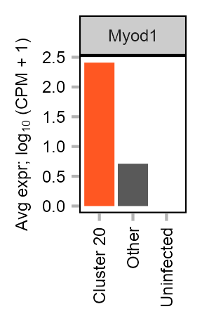
Expression of Myod1 in MEF-derived cells.
cells_barplot <- list(
    embedding |>
        dplyr::filter(
            cluster == 20 & category %in% ("JD168")
        ) |>
        dplyr::pull(cell),
    embedding |>
        dplyr::filter(
            cluster != 20 & category %in% ("JD168")
        ) |>
        dplyr::pull(cell),
    embedding |>
        dplyr::filter(
            category %in% ("JD174")
        ) |>
        dplyr::pull(cell)
)
names(cells_barplot) <- c("Cluster 20", "Other", "Uninfected")

features_barplot <- c(
    "ENSMUSG00000009471_Myod1",
    "ENSMUSG00000016458_Wt1",
    "ENSMUSG00000025105_Bnc1"
)

barplot_helper(cells_barplot, features_barplot, matrix_readcount_use) |>
    dplyr::filter(feature == "ENSMUSG00000009471_Myod1") |>
    dplyr::mutate(
        feature = stringr::str_remove(string = feature, pattern = "^.+_")
    ) |>
    dplyr::mutate(value = log10(value + 1)) |>
    plot_barplot_simple(
        x = "group",
        y = "value",
        z = "feature",
        y_title = expression("Avg expr; log"[10] * " (CPM + 1)")
    ) +
    theme_customized_violin(
        strip_background_fill = "grey80",
        panel_border_color = "black",
        axis_text_x_angle = c(90, 1, 0.5)
    ) +
    ggplot2::scale_fill_manual(
        values = c(
            c(
                "#FF5722",
                "grey35",
                "grey35"
            )
        )
    )
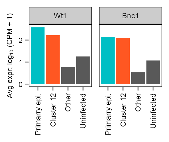
Expression of Wt1 and Bnc1 in MEF-derived cells.
cells_barplot <- list(
    embedding |>
        dplyr::filter(
            cluster == 12,
            !category %in% c("JD168", "JD174")
        ) |>
        dplyr::pull(cell),
    embedding |>
        dplyr::filter(
            cluster == 12 & category %in% ("JD168")
        ) |>
        dplyr::pull(cell),
    embedding |>
        dplyr::filter(
            cluster != 12 & category %in% ("JD168")
        ) |>
        dplyr::pull(cell),
    embedding |>
        dplyr::filter(
            category %in% ("JD174")
        ) |>
        dplyr::pull(cell)
)
names(cells_barplot) <- c("Primarry epi.", "Cluster 12", "Other", "Uninfected")

barplot_helper(cells_barplot, features_barplot, matrix_readcount_use) |>
    dplyr::filter(feature != "ENSMUSG00000009471_Myod1") |>
    dplyr::mutate(
        feature = stringr::str_remove(string = feature, pattern = "^.+_"),
        feature = factor(
            feature,
            levels = c("Wt1", "Bnc1")
        )
    ) |>
    dplyr::mutate(
        value = log10(value + 1),
        group = factor(
            group,
            levels = names(cells_barplot)
        )
    ) |>
    plot_barplot_simple(
        x = "group",
        y = "value",
        z = "feature",
        y_title = expression("Avg expr; log"[10] * " (CPM + 1)")
    ) +
    theme_customized_violin(
        strip_background_fill = "grey80",
        panel_border_color = "black",
        axis_text_x_angle = c(90, 1, 0.5)
    ) +
    ggplot2::scale_fill_manual(
        values = c(
            c(
                "#00BFC4",
                "#FF5722",
                "grey35",
                "grey35"
            )
        )
    )
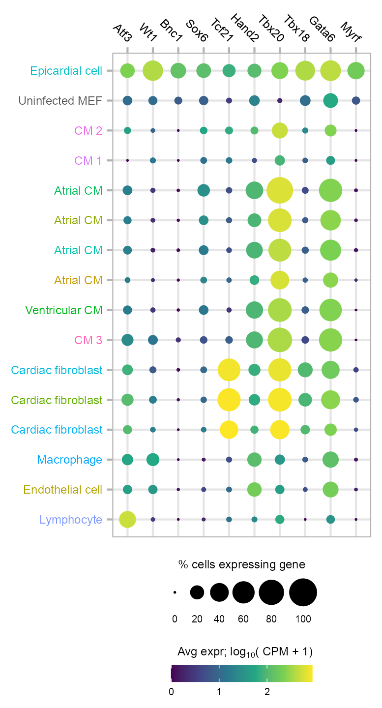
10 TFs differentially expressed in primary epicardial cells compared with uninfected MEFs. Shown is the expression of 10F in MEFs and P0 mouse heart cells.
cells_lollipop <- embedding |>
    dplyr::filter(
        !cluster %in% c(1, 2, 3, 10, 17, 20, 22),
        !category %in% c("JD168", "JD174")
    ) |>
    split(~cluster) |>
    purrr::map(\(x) {
        x |> dplyr::pull(cell)
    })

cells_lollipop <- cells_lollipop[
    purrr::map_lgl(cells_lollipop, \(x) length(x) > 0)
]

cells_lollipop$control <- embedding |>
    dplyr::filter(category %in% c("JD168", "JD174")) |>
    dplyr::pull(cell)


labels_y <- c(
    "12", "control", "19", "18", "9", "6", "11", "4", "8",
    "21", "13", "7", "14", "15", "5", "16"
)plot_lollipop(
cells = cells_lollipop[labels_y],
features = c(
"ENSMUSG00000026628_Atf3",
"ENSMUSG00000016458_Wt1",
"ENSMUSG00000025105_Bnc1",
"ENSMUSG00000051910_Sox6",
"ENSMUSG00000045680_Tcf21",
"ENSMUSG00000038193_Hand2",
"ENSMUSG00000031965_Tbx20",
"ENSMUSG00000032419_Tbx18",
"ENSMUSG00000005836_Gata6",
"ENSMUSG00000036098_Myrf"
),
matrix_cpm = calc_cpm(matrix_readcount_use)
) +
ggplot2::scale_y_discrete(
name = NULL,
labels = c(
"Epicardial cell",
"Uninfected MEF",
"CM 2",
"CM 1",
"Atrial CM",
"Atrial CM",
"Atrial CM",
"Atrial CM",
"Ventricular CM",
"CM 3",
"Cardiac fibroblast",
"Cardiac fibroblast",
"Cardiac fibroblast",
"Macrophage",
"Endothelial cell",
"Lymphocyte"
) |> rev()
) +
theme_customized_violin(
axis_text_x_angle = c(-45, 1, 0.5),
axis_text_color_y = c(color_palette, control = "grey35")[rev(labels_y)],
panel_grid_major = TRUE
) %+replace%
ggplot2::theme(
legend.margin = ggplot2::margin(
t = 0, r = 0, b = 0, l = 0, unit = "mm"
),
legend.key.size = ggplot2::unit(2.5, "mm"),
legend.key.width = ggplot2::unit(4.0, "mm"),
legend.text = ggplot2::element_text(family = "Arial", size = 5),
legend.title = ggplot2::element_text(family = "Arial", size = 6),
legend.position = "bottom",
legend.box = "vertical" # "horizontal"
) +
ggplot2::scale_size(
name = "% cells expressing gene",
breaks = seq(0, 1, .2),
labels = seq(0, 1, .2) * 100,
limits = c(0, 1),
range = c(0, 6),
guide = ggplot2::guide_legend(
title.position = "top",
title.hjust = 0.5,
label.position = "bottom",
nrow = 1,
byrow = TRUE,
order = 1
)
) +
ggplot2::scale_color_viridis_c(
name = expression(paste("Avg expr; log"[10], "( CPM + 1)")),
guide = ggplot2::guide_colourbar(
title.position = "top",
title.hjust = 1,
barwidth = 5,
barheight = 0.6,
direction = "horizontal",
order = 2
)
)
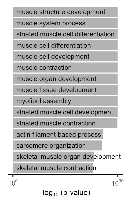
Gene ontology analysis for genes highly expressed in Cluster 20.
groupGOTerms: GOBPTerm, GOMFTerm, GOCCTerm environments built.packageVersion("topGO")[1] '2.52.0'packageVersion("org.Mm.eg.db")[1] '3.17.0'de_paired <- detect_de(
cell_group_a = embedding |>
dplyr::filter(
category == "JD168",
cluster == 20
) |>
dplyr::pull(cell),
cell_group_b = embedding |>
dplyr::filter(
category == "JD168",
cluster != 20
) |>
dplyr::pull(cell),
matrix_readcount = matrix_readcount_use,
matrix_cpm = calc_cpm(matrix_readcount_use)
# only_enrichment = TRUE
)
de_paired |> head() log2_effect pval positive_frac_a
ENSMUSG00000037139_Myom3 8.166286 3.152517e-219 0.604
ENSMUSG00000079588_Tmem182 8.050808 5.009801e-140 0.402
ENSMUSG00000026251_Chrnd 7.992256 5.311037e-81 0.238
ENSMUSG00000087591_Gm14635 7.975343 2.164927e-110 0.323
ENSMUSG00000101680_Gm29015 7.963194 4.971533e-89 0.262
ENSMUSG00000102717_Gm37759 7.876779 1.253173e-149 0.439
positive_frac_b norm_reads_mean_a norm_reads_mean_b
ENSMUSG00000037139_Myom3 0.002 1.5196756 0.0018586658
ENSMUSG00000079588_Tmem182 0.002 0.8570739 0.0008143528
ENSMUSG00000026251_Chrnd 0.001 0.2803849 0.0004863366
ENSMUSG00000087591_Gm14635 0.001 0.6266815 0.0006813209
ENSMUSG00000101680_Gm29015 0.001 0.4385369 0.0020254669
ENSMUSG00000102717_Gm37759 0.002 0.7279072 0.0018620079
log2_fc_norm_reads cpm_meam_a cpm_meam_b log2_fc_cpm
ENSMUSG00000037139_Myom3 7.011140 177.63879 0.21767902 9.607811
ENSMUSG00000079588_Tmem182 6.325136 100.13546 0.09540360 9.891957
ENSMUSG00000026251_Chrnd 4.791384 32.73270 0.05698473 8.933125
ENSMUSG00000087591_Gm14635 5.897410 73.21501 0.07976347 9.671992
ENSMUSG00000101680_Gm29015 5.221062 51.29588 0.23699159 7.698518
ENSMUSG00000102717_Gm37759 5.959019 85.12481 0.21819530 8.543336
pval_adj
ENSMUSG00000037139_Myom3 6.067921e-219
ENSMUSG00000079588_Tmem182 8.772996e-140
ENSMUSG00000026251_Chrnd 8.352273e-81
ENSMUSG00000087591_Gm14635 3.606077e-110
ENSMUSG00000101680_Gm29015 7.951628e-89
ENSMUSG00000102717_Gm37759 2.229182e-149dim(de_paired)[1] 1126 11genes_of_interest <- rownames(subset(de_paired, log2_effect > 0))
gene_universe <- rownames(matrix_readcount_use)
genes_formatted <- factor(as.integer(gene_universe %in% genes_of_interest))
names(genes_formatted) <- gene_universe
names(genes_formatted) <- names(genes_formatted) |>
stringr::str_remove(pattern = "_.+$")
topgo_data <- new(
"topGOdata",
ontology = "BP",
allGenes = genes_formatted,
annot = annFUN.org,
mapping = "org.Mm.eg.db",
ID = "Ensembl"
)
##
## Building most specific GOs .....
## Loading required package: org.Mm.eg.db
##
## ( 12764 GO terms found. )
##
## Build GO DAG topology ..........
## ( 16000 GO terms and 36196 relations. )
##
## Annotating nodes ...............
## ( 21037 genes annotated to the GO terms. )
topgo_out_classic_fisher <- topGO::runTest(
topgo_data,
algorithm = "classic",
statistic = "fisher"
)
##
## -- Classic Algorithm --
##
## the algorithm is scoring 5243 nontrivial nodes
## parameters:
## test statistic: fisherNUM_GO_TERMS <- 15
# prepare data
enriched_gos <- topGO::GenTable(topgo_data,
classicFisher = topgo_out_classic_fisher,
topNodes = NUM_GO_TERMS
) |>
dplyr::mutate(
classicFisher = as.numeric(
stringr::str_replace(classicFisher, "< ", "")
),
Term = factor(Term(GO.ID),
levels = rev(Term(GO.ID))
)
)
ggplot2::ggplot(
enriched_gos,
ggplot2::aes(
y = -log10(classicFisher),
x = Term
)
) +
ggplot2::geom_bar(stat = "identity", fill = "grey70") +
ggplot2::coord_flip() +
ggplot2::labs(x = NULL) +
ggplot2::theme_classic() +
ggplot2::scale_y_continuous(
name = expression(paste("-log"[10], " (p-value)")),
breaks = c(0, 30),
labels = scales::math_format(10^.x)
) +
ggplot2::annotate(
geom = "text",
x = seq_len(nrow(enriched_gos)),
y = rep(1, nrow(enriched_gos)),
label = rev(enriched_gos$Term),
# vjust = "inward",
hjust = "inward",
size = 2.5,
family = "Arial"
) +
ggplot2::theme(
axis.title = ggplot2::element_text(family = "Arial", size = 8),
axis.title.y = ggplot2::element_blank(),
axis.text = ggplot2::element_text(family = "Arial", size = 7),
axis.text.y = ggplot2::element_blank(),
axis.ticks.y = ggplot2::element_blank(),
axis.line.y = ggplot2::element_blank(),
legend.text = ggplot2::element_text(family = "Arial", size = 8),
legend.title = ggplot2::element_text(family = "Arial", size = 8)
)
# clusters_selected <- c(1, 2, 3, 10, 12, 17, 20, 22)

features_selected_43 <- c(
    "ENSMUSG00000025930_Msc",
    "ENSMUSG00000026313_Hdac4",
    "ENSMUSG00000026565_Pou2f1",
    "ENSMUSG00000026923_Notch1",
    "ENSMUSG00000015846_Rxra",
    "ENSMUSG00000015627_Gata5",
    "ENSMUSG00000025860_Xiap",
    "ENSMUSG00000040289_Hey1",
    "ENSMUSG00000027833_Shox2",
    "ENSMUSG00000001419_Mef2d",
    "ENSMUSG00000028800_Hdac1",
    "ENSMUSG00000086369_E330017L17Rik",
    "ENSMUSG00000028949_Smarcd3",
    "ENSMUSG00000048450_Msx1",
    "ENSMUSG00000042002_Foxn4",
    "ENSMUSG00000018604_Tbx3",
    "ENSMUSG00000018263_Tbx5",
    "ENSMUSG00000063568_Jazf1",
    "ENSMUSG00000009471_Myod1",
    "ENSMUSG00000030557_Mef2a",
    "ENSMUSG00000030551_Nr2f2",
    "ENSMUSG00000030544_Mesp1",
    "ENSMUSG00000019789_Hey2",
    "ENSMUSG00000019777_Hdac2",
    "ENSMUSG00000020167_Tcf3",
    "ENSMUSG00000038193_Hand2",
    "ENSMUSG00000079033_Mef2b",
    "ENSMUSG00000021944_Gata4",
    "ENSMUSG00000032419_Tbx18",
    "ENSMUSG00000020160_Meis1",
    "ENSMUSG00000037335_Hand1",
    "ENSMUSG00000020542_Myocd",
    "ENSMUSG00000000093_Tbx2",
    "ENSMUSG00000021469_Msx2",
    "ENSMUSG00000005583_Mef2c",
    "ENSMUSG00000042258_Isl1",
    "ENSMUSG00000009739_Pou6f1",
    "ENSMUSG00000001288_Rarg",
    "ENSMUSG00000015579_Nkx2-5",
    "ENSMUSG00000023067_Cdkn1a",
    "ENSMUSG00000024063_Lbh",
    "ENSMUSG00000005836_Gata6",
    "ENSMUSG00000024515_Smad4"
)
clusters_selected <- c(20, 12, 2)
enriched_factors <- do.call(
rbind.data.frame,
lapply(clusters_selected, \(x) {
cells_1 <- embedding$cell[
embedding$cluster == x & embedding$category == "JD168"
]
cells_2 <- embedding$cell[
embedding$cluster != x & embedding$category == "JD168"
]
cat(x, length(cells_1), length(cells_2), "\n")
de_paired <- detect_de(
cell_group_a = cells_1,
cell_group_b = cells_2,
matrix_readcount = matrix_readcount_use,
matrix_cpm = calc_cpm(matrix_readcount_use),
only_enrichment = TRUE
) |>
dplyr::mutate(category = x) |>
tibble::rownames_to_column(var = "feature") |>
dplyr::filter(feature %in% features_selected_43)
})
) |>
dplyr::filter(category %in% clusters_selected) |>
dplyr::mutate(
category = factor(category,
levels = clusters_selected
),
symbol = stringr::str_remove(
string = feature,
pattern = "^.+_"
)
)20 164 8566
12 201 8529
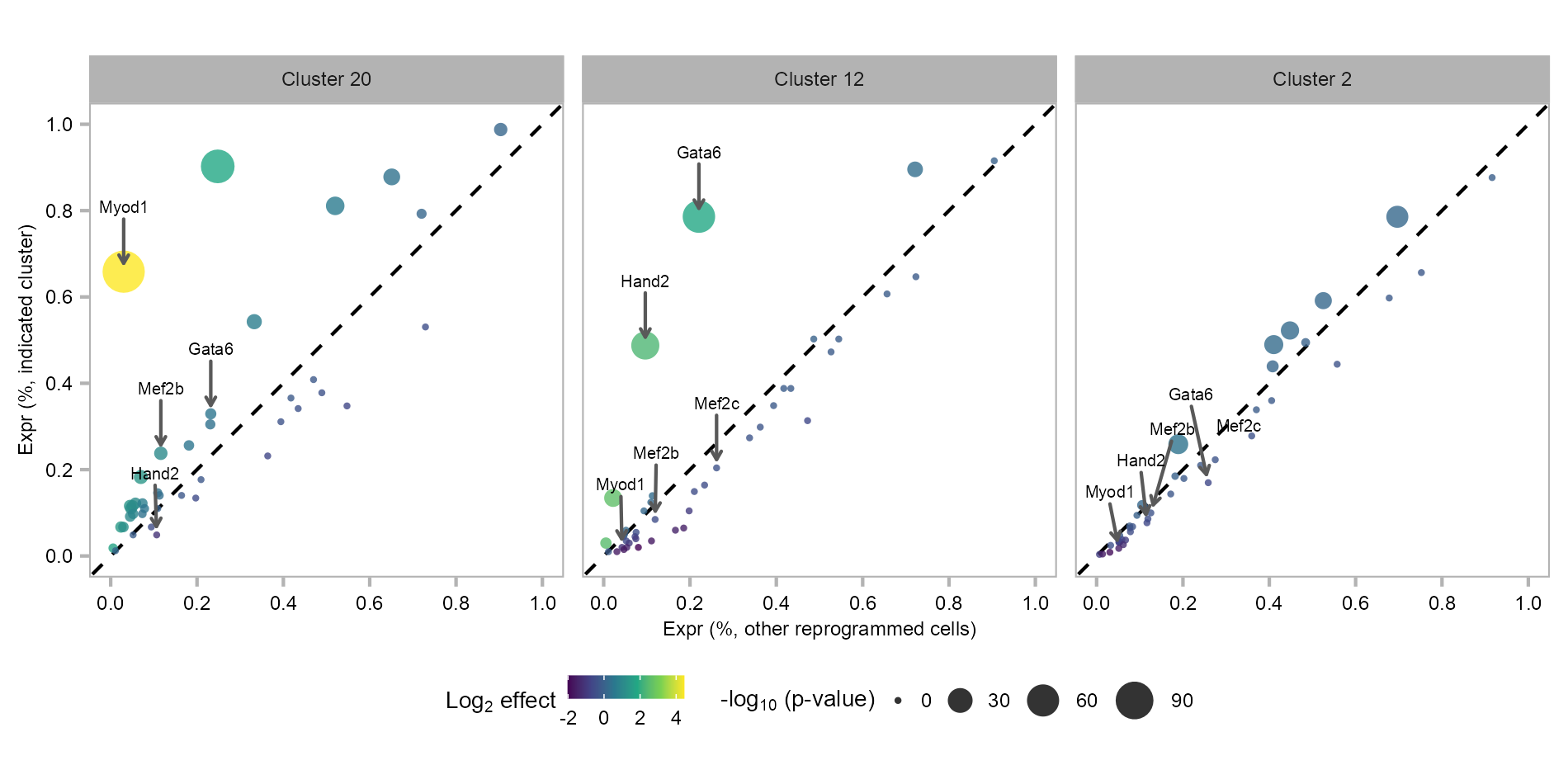
2 2445 6285 Differential expression analysis of 48F in MEF-derived clusters, as compared with all other reprogrammed cells. Each dot represents a gene (colored by fold change and sized by p value).
ggplot2::ggplot() +
    ggplot2::geom_abline(intercept = 0, slope = 1, linetype = 2) +
    ggplot2::geom_point(
        data = enriched_factors,
        ggplot2::aes(positive_frac_b,
            positive_frac_a,
            size = -log10(pval_adj),
            color = log2_effect
        ),
        alpha = .8,
        stroke = 0, shape = 16
    ) +
    ggplot2::facet_wrap(
        ~category,
        nrow = 1,
        labeller = ggplot2::labeller(
            category = setNames(
                object = paste("Cluster", clusters_selected),
                nm = clusters_selected
            )
        )
    ) +
    ggplot2::coord_fixed() +
    ggplot2::scale_color_viridis_c(
        name = expression(paste("Log"[2], " effect"))
    ) +
    ggplot2::scale_size_continuous(
        name = expression(paste("-log"[10], " (p-value)"))
    ) +
    ggplot2::guides(
        color = ggplot2::guide_colorbar(order = 1),
        size = ggplot2::guide_legend(order = 2)
    ) +
    ggplot2::scale_x_continuous(
        name = "Expr (%, other reprogrammed cells)",
        limits = c(0, 1), breaks = seq(0, 1, .2)
    ) +
    ggplot2::scale_y_continuous(
        name = "Expr (%, indicated cluster)",
        limits = c(0, 1), breaks = seq(0, 1, .2)
    ) +
    theme_customized_violin() %+replace%
    ggplot2::theme(
        legend.background = ggplot2::element_blank(),
        legend.margin = ggplot2::margin(t = 0, r = 0, b = 0, l = 0, unit = "mm"),
        legend.key.size = ggplot2::unit(2.5, "mm"),
        legend.text = ggplot2::element_text(family = "Arial", size = 6),
        legend.title = ggplot2::element_text(family = "Arial", size = 7),
        legend.position = "bottom",
        legend.box = "horizontal",
        legend.box.background = ggplot2::element_blank()
    ) +
    ggrepel::geom_text_repel(
        data = subset(enriched_factors, symbol %in% c(
            "Myod1", "Mef2b",
            "Mef2c", "Hand2", "Gata6"
        )),
        ggplot2::aes(
            positive_frac_b,
            positive_frac_a,
            label = symbol
        ),
        #
        size = 5 / ggplot2::.pt,
        family = "Arial",
        box.padding = .2,
        point.padding = .2,
        nudge_y = .15,
        arrow = ggplot2::arrow(length = ggplot2::unit(.02, "npc")),
        segment.color = "grey35",
        color = "black"
    )
devtools::session_info()─ Session info ───────────────────────────────────────────────────────────────
setting value
version R version 4.3.1 (2023-06-16)
os macOS Ventura 13.5
system aarch64, darwin22.4.0
ui unknown
language (EN)
collate en_US.UTF-8
ctype en_US.UTF-8
tz America/Chicago
date 2023-08-12
pandoc 2.19.2 @ /Users/jialei/.pyenv/shims/ (via rmarkdown)
─ Packages ───────────────────────────────────────────────────────────────────
package * version date (UTC) lib source
AnnotationDbi * 1.62.2 2023-07-02 [1] Bioconductor
Biobase * 2.60.0 2023-04-25 [1] Bioconductor
BiocGenerics * 0.46.0 2023-04-25 [1] Bioconductor
Biostrings 2.68.1 2023-05-16 [1] Bioconductor
bit 4.0.5 2022-11-15 [1] CRAN (R 4.3.0)
bit64 4.0.5 2020-08-30 [1] CRAN (R 4.3.0)
bitops 1.0-7 2021-04-24 [1] CRAN (R 4.3.0)
blob 1.2.4 2023-03-17 [1] CRAN (R 4.3.0)
cachem 1.0.8 2023-05-01 [1] CRAN (R 4.3.0)
callr 3.7.3 2022-11-02 [1] CRAN (R 4.3.0)
cli 3.6.1 2023-03-23 [1] CRAN (R 4.3.0)
colorspace 2.1-0 2023-01-23 [1] CRAN (R 4.3.0)
commonmark 1.9.0 2023-03-17 [1] CRAN (R 4.3.0)
crayon 1.5.2 2022-09-29 [1] CRAN (R 4.3.0)
DBI 1.1.3 2022-06-18 [1] CRAN (R 4.3.0)
devtools 2.4.5.9000 2023-08-11 [1] Github (r-lib/devtools@163c3f2)
digest 0.6.33 2023-07-07 [1] CRAN (R 4.3.1)
dplyr * 1.1.2.9000 2023-07-19 [1] Github (tidyverse/dplyr@c963d4d)
ellipsis 0.3.2 2021-04-29 [1] CRAN (R 4.3.0)
evaluate 0.21 2023-05-05 [1] CRAN (R 4.3.0)
extrafont * 0.19 2023-01-18 [1] CRAN (R 4.3.0)
extrafontdb 1.0 2012-06-11 [1] CRAN (R 4.3.0)
fansi 1.0.4 2023-01-22 [1] CRAN (R 4.3.0)
farver 2.1.1 2022-07-06 [1] CRAN (R 4.3.0)
fastmap 1.1.1 2023-02-24 [1] CRAN (R 4.3.0)
forcats * 1.0.0.9000 2023-04-23 [1] Github (tidyverse/forcats@4a8525a)
formattable * 0.2.1 2021-01-07 [1] CRAN (R 4.3.1)
fs 1.6.3 2023-07-20 [1] CRAN (R 4.3.1)
generics 0.1.3 2022-07-05 [1] CRAN (R 4.3.0)
GenomeInfoDb 1.36.1 2023-06-21 [1] Bioconductor
GenomeInfoDbData 1.2.10 2023-04-23 [1] Bioconductor
ggplot2 * 3.4.2.9000 2023-08-11 [1] Github (tidyverse/ggplot2@2cd0e96)
ggrepel 0.9.3 2023-02-03 [1] CRAN (R 4.3.0)
glue 1.6.2.9000 2023-04-23 [1] Github (tidyverse/glue@cbac82a)
GO.db * 3.17.0 2023-04-24 [1] Bioconductor
graph * 1.78.0 2023-04-25 [1] Bioconductor
gt 0.9.0.9000 2023-08-11 [1] Github (rstudio/gt@a3cc005)
gtable 0.3.3.9000 2023-04-23 [1] Github (r-lib/gtable@c56fd4f)
hms 1.1.3 2023-03-21 [1] CRAN (R 4.3.0)
htmltools 0.5.6 2023-08-10 [1] CRAN (R 4.3.1)
htmlwidgets 1.6.2 2023-03-17 [1] CRAN (R 4.3.0)
httr 1.4.6 2023-05-08 [1] CRAN (R 4.3.0)
IRanges * 2.34.1 2023-06-22 [1] Bioconductor
jsonlite 1.8.7 2023-06-29 [1] CRAN (R 4.3.1)
KEGGREST 1.40.0 2023-04-25 [1] Bioconductor
knitr 1.43 2023-05-25 [1] CRAN (R 4.3.0)
labeling 0.4.2 2020-10-20 [1] CRAN (R 4.3.0)
lattice 0.21-8 2023-04-05 [2] CRAN (R 4.3.1)
lifecycle 1.0.3 2022-10-07 [1] CRAN (R 4.3.0)
lubridate * 1.9.2.9000 2023-07-22 [1] Github (tidyverse/lubridate@cae67ea)
magrittr 2.0.3 2022-03-30 [1] CRAN (R 4.3.0)
markdown 1.7 2023-05-16 [1] CRAN (R 4.3.0)
Matrix * 1.6-0 2023-07-08 [2] CRAN (R 4.3.1)
matrixStats 1.0.0 2023-06-02 [1] CRAN (R 4.3.0)
memoise 2.0.1 2021-11-26 [1] CRAN (R 4.3.0)
munsell 0.5.0 2018-06-12 [1] CRAN (R 4.3.0)
org.Mm.eg.db * 3.17.0 2023-07-22 [1] Bioconductor
patchwork * 1.1.2.9000 2023-08-11 [1] Github (thomasp85/patchwork@bd57553)
pillar 1.9.0 2023-03-22 [1] CRAN (R 4.3.0)
pkgbuild 1.4.2 2023-06-26 [1] CRAN (R 4.3.1)
pkgconfig 2.0.3 2019-09-22 [1] CRAN (R 4.3.0)
pkgload 1.3.2.9000 2023-07-05 [1] Github (r-lib/pkgload@3cf9896)
png 0.1-8 2022-11-29 [1] CRAN (R 4.3.0)
prettyunits 1.1.1.9000 2023-04-23 [1] Github (r-lib/prettyunits@8706d89)
processx 3.8.2 2023-06-30 [1] CRAN (R 4.3.1)
ps 1.7.5 2023-04-18 [1] CRAN (R 4.3.0)
purrr * 1.0.2.9000 2023-08-11 [1] Github (tidyverse/purrr@ac4f5a9)
R.cache 0.16.0 2022-07-21 [1] CRAN (R 4.3.0)
R.methodsS3 1.8.2 2022-06-13 [1] CRAN (R 4.3.0)
R.oo 1.25.0 2022-06-12 [1] CRAN (R 4.3.0)
R.utils 2.12.2 2022-11-11 [1] CRAN (R 4.3.0)
R6 2.5.1.9000 2023-04-23 [1] Github (r-lib/R6@e97cca7)
ragg 1.2.5 2023-01-12 [1] CRAN (R 4.3.0)
Rcpp 1.0.11 2023-07-06 [1] CRAN (R 4.3.1)
RCurl 1.98-1.12 2023-03-27 [1] CRAN (R 4.3.0)
readr * 2.1.4.9000 2023-08-03 [1] Github (tidyverse/readr@80e4dc1)
remotes 2.4.2.9000 2023-06-09 [1] Github (r-lib/remotes@8875171)
rlang 1.1.1.9000 2023-06-09 [1] Github (r-lib/rlang@c55f602)
rmarkdown 2.23.4 2023-07-27 [1] Github (rstudio/rmarkdown@054d735)
RSQLite 2.3.1 2023-04-03 [1] CRAN (R 4.3.0)
rstudioapi 0.15.0.9000 2023-07-19 [1] Github (rstudio/rstudioapi@feceaef)
Rttf2pt1 1.3.12 2023-01-22 [1] CRAN (R 4.3.0)
S4Vectors * 0.38.1 2023-05-02 [1] Bioconductor
sass 0.4.7 2023-07-15 [1] CRAN (R 4.3.1)
scales 1.2.1 2022-08-20 [1] CRAN (R 4.3.0)
sessioninfo 1.2.2 2021-12-06 [1] CRAN (R 4.3.0)
SparseM * 1.81 2021-02-18 [1] CRAN (R 4.3.1)
stringi 1.7.12 2023-01-11 [1] CRAN (R 4.3.0)
stringr * 1.5.0.9000 2023-08-11 [1] Github (tidyverse/stringr@08ff36f)
styler * 1.10.1 2023-07-17 [1] Github (r-lib/styler@aca7223)
systemfonts 1.0.4 2022-02-11 [1] CRAN (R 4.3.0)
textshaping 0.3.6 2021-10-13 [1] CRAN (R 4.3.0)
tibble * 3.2.1.9005 2023-05-28 [1] Github (tidyverse/tibble@4de5c15)
tidyr * 1.3.0.9000 2023-04-23 [1] Github (tidyverse/tidyr@0764e65)
tidyselect 1.2.0 2022-10-10 [1] CRAN (R 4.3.0)
tidyverse * 2.0.0.9000 2023-04-23 [1] Github (tidyverse/tidyverse@8ec2e1f)
timechange 0.2.0 2023-01-11 [1] CRAN (R 4.3.0)
topGO * 2.52.0 2023-04-25 [1] Bioconductor
tzdb 0.4.0 2023-05-12 [1] CRAN (R 4.3.0)
usethis 2.2.2.9000 2023-07-11 [1] Github (r-lib/usethis@467ff57)
utf8 1.2.3 2023-01-31 [1] CRAN (R 4.3.0)
vctrs 0.6.3 2023-06-14 [1] CRAN (R 4.3.0)
viridisLite 0.4.2 2023-05-02 [1] CRAN (R 4.3.0)
vroom 1.6.3.9000 2023-04-30 [1] Github (tidyverse/vroom@89b6aac)
withr 2.5.0 2022-03-03 [1] CRAN (R 4.3.0)
xfun 0.40 2023-08-09 [1] CRAN (R 4.3.1)
xml2 1.3.5 2023-07-06 [1] CRAN (R 4.3.1)
XVector 0.40.0 2023-04-25 [1] Bioconductor
yaml 2.3.7 2023-01-23 [1] CRAN (R 4.3.0)
zlibbioc 1.46.0 2023-04-25 [1] Bioconductor
[1] /opt/homebrew/lib/R/4.3/site-library
[2] /opt/homebrew/Cellar/r/4.3.1/lib/R/library
──────────────────────────────────────────────────────────────────────────────Styling 1 files:
unbiased_reprogramming.qmd ✔
────────────────────────────────────────
Status Count Legend
✔ 1 File unchanged.
ℹ 0 File changed.
✖ 0 Styling threw an error.
────────────────────────────────────────@article{duan2023,
author = {Duan, Jialei and Li, Boxun and Bhakta, Minoti and Xie, Shiqi
and Zhou, Pei and V. Munshi, Nikhil and C. Hon, Gary},
publisher = {Cell Press},
title = {Rational {Reprogramming} of {Cellular} {States} by
{Combinatorial} {Perturbation}},
journal = {Cell reports},
volume = {27},
number = {12},
pages = {3486 - 3499000000},
date = {2023-08-12},
url = {https://doi.org/10.1016/j.celrep.2019.05.079},
doi = {10.1016/j.celrep.2019.05.079},
langid = {en},
abstract = {Reprogram-Seq leverages organ-specific cell atlas data
with single-cell perturbation and computational analysis to predict,
evaluate, and optimize TF combinations that reprogram a cell type of
interest.}
}