Single Cell Transcriptomes of Human Blastoids
Jialei Duan 
Abstract
Human blastoids provide a readily accessible, scalable, versatile and perturbable alternative to blastocysts for studying early human development, understanding early pregnancy loss and gaining insights into early developmental defects.
Sys.time()[1] "2022-09-25 00:33:35 CDT"[1] "America/Chicago"Preparation
Functions
Load required packages.
source(
    file = file.path(
        SCRIPT_DIR,
        "utilities.R"
    )
)

load_matrix <- function(x) {
    matrix_readcount_use <- scipy.sparse$load_npz(
        file.path(x, "matrix_readcount.npz")
    )
    colnames(matrix_readcount_use) <- np$load(
        file.path(x, "matrix_readcount_barcodes.npy")
    )
    rownames(matrix_readcount_use) <- np$load(
        file.path(x, "matrix_readcount_features.npy")
    )

    return(matrix_readcount_use)
}
Python env
reticulate::py_config()python: /Users/jialei/.pyenv/shims/python
libpython: /Users/jialei/.pyenv/versions/mambaforge-4.10.3-10/lib/libpython3.9.dylib
pythonhome: /Users/jialei/.pyenv/versions/mambaforge-4.10.3-10:/Users/jialei/.pyenv/versions/mambaforge-4.10.3-10
version: 3.9.13 | packaged by conda-forge | (main, May 27 2022, 17:00:33) [Clang 13.0.1 ]
numpy: /Users/jialei/.pyenv/versions/mambaforge-4.10.3-10/lib/python3.9/site-packages/numpy
numpy_version: 1.22.4
numpy: /Users/jialei/.pyenv/versions/mambaforge-4.10.3-10/lib/python3.9/site-packages/numpy
NOTE: Python version was forced by RETICULATE_PYTHONMatrix
PROJECT_DIR <- "/Users/jialei/Dropbox/Data/Projects/UTSW/Human_blastoid"MATRIX_DIR <- list(
"github/data/matrices/LW36",
"github/data/matrices/LW49_LW50_LW51_LW52",
"github/data/matrices/LW58_LW59",
"github/data/matrices/LW60_LW61",
"raw/public/PRJEB11202/reformatted_matrix"
)
matrix_readcount_use <- purrr::map(MATRIX_DIR, \(x) {
load_matrix(file.path(PROJECT_DIR, x))
}) |>
purrr::reduce(cbind)
# clean up
rm(MATRIX_DIR)Embedding
Metadata
cell_metadata_PRJEB11202 <- read_delim(
file.path(
PROJECT_DIR,
"raw/public/PRJEB11202/",
"E-MTAB-3929.sdrf.tsv"
),
delim = "\t"
) |>
dplyr::select(
`Comment[ENA_SAMPLE]`,
`Comment[ENA_RUN]`,
`Characteristics[developmental stage]`,
`Characteristics[inferred lineage]`
) |>
dplyr::rename(
cell = `Comment[ENA_SAMPLE]`,
run = `Comment[ENA_RUN]`,
developmental_stage = `Characteristics[developmental stage]`,
lineage = `Characteristics[inferred lineage]`
) |>
dplyr::mutate(
developmental_stage = str_replace(
string = developmental_stage,
pattern = "embryonic day ",
replacement = "E"
),
lineage = case_when(
lineage == "epiblast" ~ "EPI",
lineage == "primitive endoderm" ~ "HYP",
lineage == "trophectoderm" ~ "TE",
lineage == "not applicable" ~ "Pre-lineage"
)
)
embedding <- embedding |>
dplyr::left_join(
cell_metadata_PRJEB11202
) |>
dplyr::mutate(
developmental_stage = factor(developmental_stage),
lineage = factor(lineage)
)Check memory usage.
walk(list(matrix_readcount_use, embedding), \(x) {
print(object.size(x), units = "auto", standard = "SI")
})496.5 MB
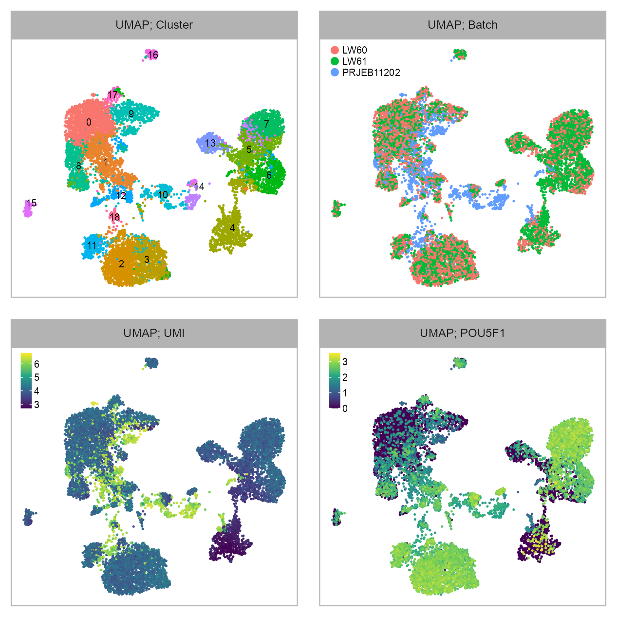
1.6 MBBlastoids globally resemble blastocysts
Embedding visualization
EMBEDDING_TITLE_PREFIX <- "UMAP"
x_column <- "x_umap"
y_column <- "y_umap"
GEOM_POINT_SIZE <- 0.6
RASTERISED <- FALSEClustering & batch & UMI
p_embedding_louvain <- plot_embedding(
data = embedding[, c(x_column, y_column)],
color = embedding$louvain |> as.factor(),
label = glue::glue("{EMBEDDING_TITLE_PREFIX}; Cluster"),
color_labels = TRUE,
color_legend = FALSE,
sort_values = FALSE,
shuffle_values = TRUE,
rasterise = RASTERISED,
geom_point_size = GEOM_POINT_SIZE
) +
theme_customized_embedding()
p_embedding_batch <- plot_embedding(
data = embedding[, c(x_column, y_column)],
color = embedding$batch |> as.factor(),
label = glue::glue("{EMBEDDING_TITLE_PREFIX}; Batch"),
color_labels = FALSE,
color_legend = TRUE,
sort_values = FALSE,
shuffle_values = TRUE,
rasterise = RASTERISED,
geom_point_size = GEOM_POINT_SIZE
) +
theme_customized_embedding()
p_embedding_UMI <- plot_embedding(
data = embedding[, c(x_column, y_column)],
color = log10(Matrix::colSums(matrix_readcount_use[, embedding$cell])),
label = glue::glue("{EMBEDDING_TITLE_PREFIX}; UMI"),
color_legend = TRUE,
sort_values = FALSE,
shuffle_values = TRUE,
rasterise = RASTERISED,
geom_point_size = GEOM_POINT_SIZE
) +
theme_customized_embedding()
selected_feature <- "ENSG00000204531_POU5F1"
p_embedding_POU5F1 <- plot_embedding(
data = embedding[, c(x_column, y_column)],
color = log10(
calc_cpm(matrix_readcount_use[, embedding$cell])
[selected_feature, ] + 1
),
label = glue::glue(
"{EMBEDDING_TITLE_PREFIX}; ",
"{selected_feature |> stringr::str_remove(pattern = \"^E.+_\")}"
),
color_legend = TRUE,
sort_values = TRUE,
rasterise = RASTERISED,
geom_point_size = GEOM_POINT_SIZE,
na_value = "grey80"
) +
theme_customized_embedding()embedding |>
dplyr::mutate(
num_umis = colSums(matrix_readcount_use[, cell]),
num_features = colSums(matrix_readcount_use[, cell] > 0),
) |>
dplyr::group_by(louvain) |>
dplyr::summarise(
num_cells = n(),
median_umis = median(num_umis),
median_features = median(num_features)
) |>
gt::gt() |>
gt::data_color(
columns = c(median_umis),
colors = scales::col_numeric(
palette = c(
"green", "orange", "red"
),
domain = c(1000, 32000)
)
) |>
gt::summary_rows(
columns = c(louvain),
fns = list(
Count = ~ n()
),
decimals = 0
) |>
gt::summary_rows(
columns = c(median_umis:median_features),
fns = list(
Mean = ~ mean(.)
),
decimals = 0
) |>
gt::summary_rows(
columns = c(num_cells),
fns = list(
Sum = ~ sum(.)
),
decimals = 0
) |>
gt::tab_header(
title = gt::md("**Blastoid Clustering**; Cluster")
)| Blastoid Clustering; Cluster | ||||
| louvain | num_cells | median_umis | median_features | |
|---|---|---|---|---|
| 0 | 1533 | 11534.0 | 3074.0 | |
| 1 | 1113 | 18092.0 | 3612.0 | |
| 2 | 1079 | 11308.0 | 2940.0 | |
| 3 | 996 | 14659.0 | 3220.5 | |
| 4 | 924 | 1108.5 | 627.0 | |
| 5 | 725 | 6915.0 | 1981.0 | |
| 6 | 710 | 9711.5 | 2158.0 | |
| 7 | 672 | 10544.0 | 2791.5 | |
| 8 | 649 | 11961.0 | 2905.0 | |
| 9 | 570 | 19201.0 | 3656.0 | |
| 10 | 410 | 23705.5 | 4208.5 | |
| 11 | 366 | 13910.5 | 3355.5 | |
| 12 | 365 | 16942.0 | 3437.0 | |
| 13 | 275 | 8010.0 | 2455.0 | |
| 14 | 249 | 31950.0 | 4954.0 | |
| 15 | 202 | 8217.0 | 2452.0 | |
| 16 | 138 | 10242.5 | 2852.5 | |
| 17 | 120 | 17426.0 | 3400.0 | |
| 18 | 86 | 18158.0 | 3853.5 | |
| Count | 19 | — | — | — |
| Mean | — | — | 13,873 | 3,049 |
| Sum | — | 11,182 | — | — |
embedding |>
dplyr::mutate(
num_umis = colSums(matrix_readcount_use[, cell]),
num_features = colSums(matrix_readcount_use[, cell] > 0),
) |>
dplyr::group_by(batch) |>
dplyr::summarise(
num_cells = n(),
median_umis = median(num_umis),
median_features = median(num_features)
) |>
dplyr::mutate(
sample = dplyr::case_when(
batch == "PRJEB11202" ~ "Petropoulos et al., 2016",
batch == "LW60" ~ "Blastoid, D9; HT; 5i/L/A",
batch == "LW61" ~ "Blastoid, D9; HT; 5i/L/A"
)
) |>
dplyr::select(
sample, dplyr::everything()
) |>
gt::gt() |>
gt::data_color(
columns = c(median_umis),
colors = scales::col_numeric(
palette = c(
"green", "orange", "red"
),
domain = c(7000, 1600000)
)
) |>
gt::summary_rows(
columns = c(sample:batch),
fns = list(
Count = ~ n()
),
decimals = 0
) |>
gt::summary_rows(
columns = c(median_umis:median_features),
fns = list(
Mean = ~ mean(.)
),
decimals = 0
) |>
gt::summary_rows(
columns = c(num_cells),
fns = list(
Sum = ~ sum(.)
),
decimals = 0
) |>
gt::tab_header(
title = gt::md("**Blastoid Clustering**; Batch")
)| Blastoid Clustering; Batch | |||||
| sample | batch | num_cells | median_umis | median_features | |
|---|---|---|---|---|---|
| Blastoid, D9; HT; 5i/L/A | LW60 | 4497 | 14421 | 3337 | |
| Blastoid, D9; HT; 5i/L/A | LW61 | 5156 | 7625 | 2185 | |
| Petropoulos et al., 2016 | PRJEB11202 | 1529 | 1551093 | 10305 | |
| Count | 3 | 3 | — | — | — |
| Mean | — | — | — | 524,380 | 5,276 |
| Sum | — | — | 11,182 | — | — |
purrr::reduce(list(
p_embedding_louvain,
p_embedding_batch,
p_embedding_UMI,
p_embedding_POU5F1
), `+`) +
patchwork::plot_layout(ncol = 2) +
patchwork::plot_annotation(
theme = ggplot2::theme(plot.margin = ggplot2::margin())
)
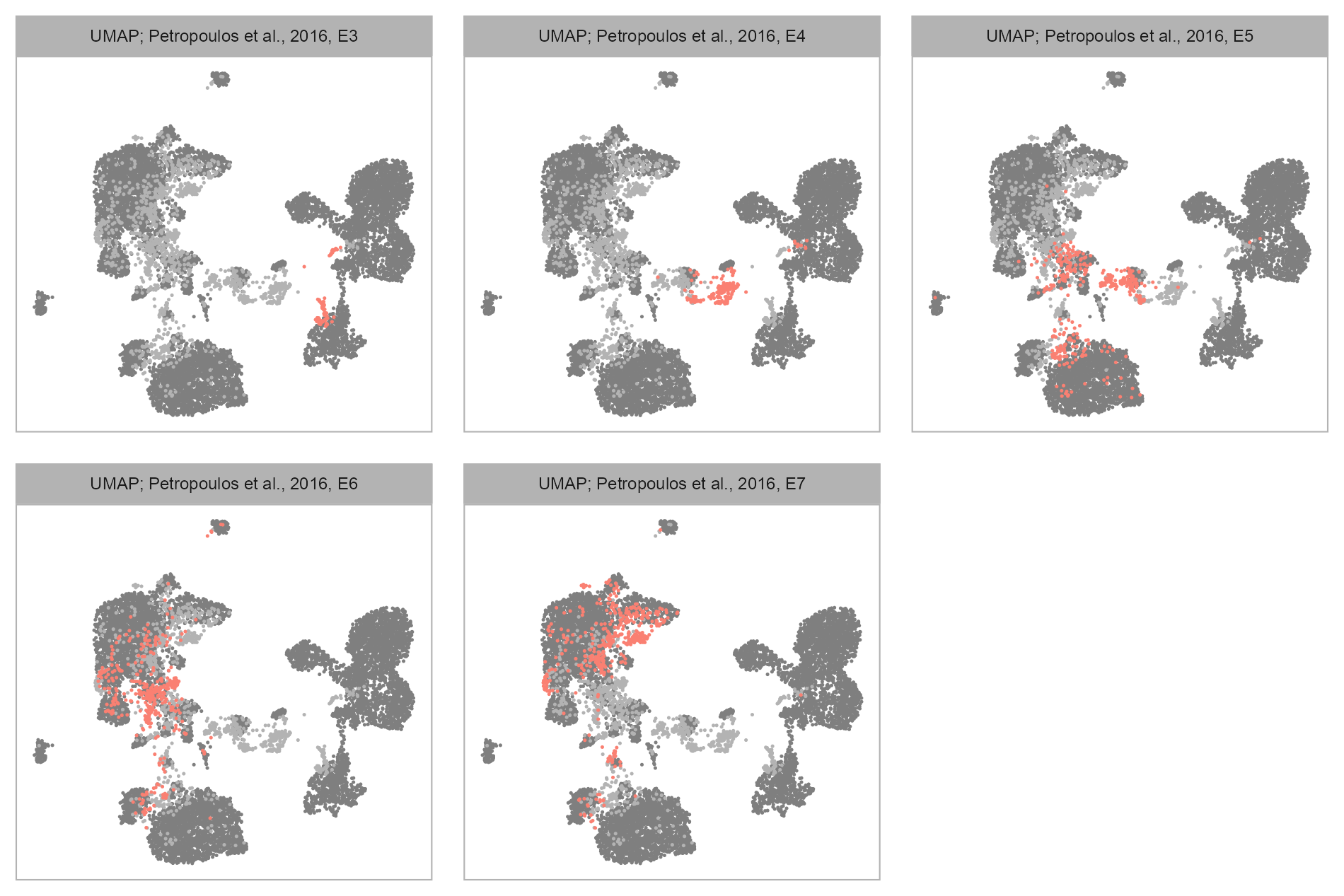
Developmental stages
Salmon: highlighted group of cells; Light grey: cells belonging to this dataset but not the highlighted group; Dark grey: cells belonging to other datasets.
purrr::map(levels(embedding$developmental_stage), \(x) {
plot_embedding(
data = embedding[, c(x_column, y_column)],
color = as.integer(embedding$developmental_stage == x) |> as.factor(),
label = glue::glue(
"{EMBEDDING_TITLE_PREFIX}; Petropoulos et al., 2016, {x}"
),
color_legend = FALSE,
sort_values = TRUE,
geom_point_size = GEOM_POINT_SIZE,
) +
theme_customized_embedding() +
ggplot2::scale_color_manual(values = c("grey70", "salmon"))
}) |>
purrr::reduce(`+`) +
patchwork::plot_layout(ncol = 3, byrow = TRUE) +
patchwork::plot_annotation(
theme = ggplot2::theme(plot.margin = ggplot2::margin())
)
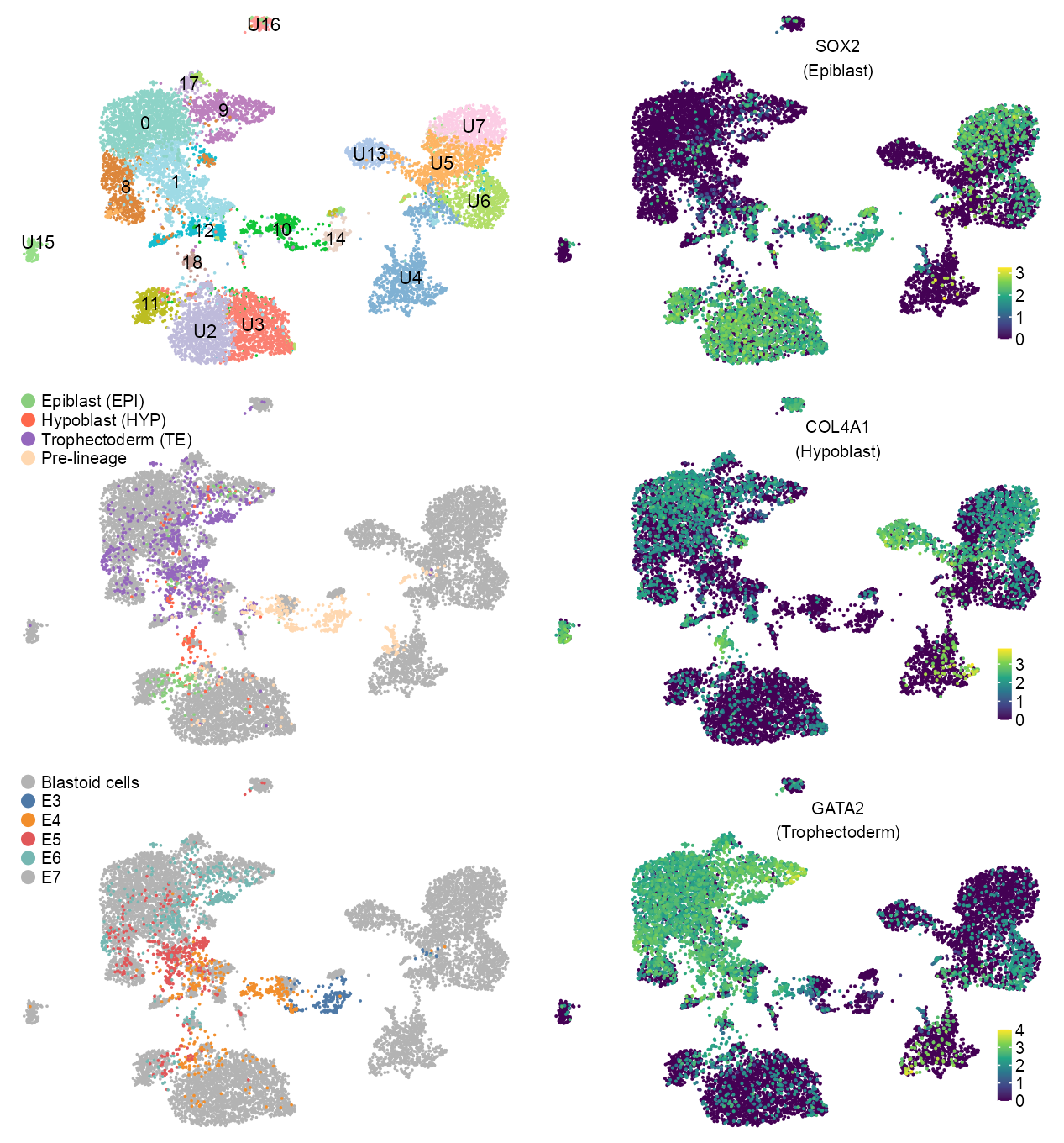
Polishing
color_palette_cluster <- c(
"0" = "#8DD3C7",
"1" = "#9EDAE5FF",
"2" = "#BEBADA",
"3" = "#FB8072",
"4" = "#80B1D3",
"5" = "#FDB462",
"6" = "#B3DE69",
"7" = "#FCCDE5",
"8" = "#DC863B",
"9" = "#BC80BD",
"10" = "#11c638",
"11" = "#BCBD22FF",
"12" = "#17BECFFF",
"13" = "#AEC7E8FF",
"14" = "#EAD3C6",
"15" = "#98DF8AFF",
"16" = "#FF9896FF",
"17" = "#C5B0D5FF",
"18" = "#C49C94FF",
"19" = "#F7B6D2FF",
"20" = "#D33F6A",
"21" = "#8E063B",
"22" = "#023FA5"
)
cluster_labels <- embedding |>
dplyr::group_by(.data[["louvain"]]) |>
dplyr::summarise(
x = quantile(.data[[x_column]], 0.5),
y = quantile(.data[[y_column]], 0.5),
.groups = "drop"
) |>
as.data.frame()
cluster_labels[cluster_labels[["louvain"]] == 14, c("x", "y")] <- c(6.8, -1.8)
clusters_unidentified <- c(2, 3, 4, 5, 6, 7, 13, 15, 16)
cluster_labels <- cluster_labels |>
dplyr::mutate(
label = dplyr::case_when(
louvain %in% clusters_unidentified ~ paste0(
"U",
as.character(louvain)
),
TRUE ~ as.character(louvain)
)
)
# cluster
p_embedding_cluster <- embedding |>
arrange(desc(louvain)) |>
ggplot(
aes(
x = .data[[x_column]],
y = .data[[y_column]],
color = .data[["louvain"]] |> as.factor()
)
) +
geom_point(
size = 0.45,
alpha = 1,
stroke = 0,
shape = 16
) +
scale_color_manual(
values = color_palette_cluster
) +
theme_void() +
ggplot2::guides(color = "none") +
ggplot2::annotate(
"text",
family = "Arial",
x = cluster_labels[, "x"],
y = cluster_labels[, "y"],
label = cluster_labels[, "label"],
parse = TRUE,
size = 2,
color = c("black")
)
# lineage
p_embedding_lineage <- plot_embedding(
data = embedding[, c(x_column, y_column)],
color = embedding |>
dplyr::mutate(
value = factor(lineage,
levels = c("Blastoid", "TE", "HYP", "EPI", "Pre-lineage")
)
) |>
dplyr::pull(value),
label = NULL,
color_legend = TRUE,
sort_values = TRUE,
geom_point_size = 0.45,
) +
theme_customized_embedding(void = TRUE) +
ggplot2::scale_color_manual(
name = NULL,
values = c("grey70", "#8ace7e", "#ff684c", "#9467bd", "#ffd8b1"),
breaks = c("Blastoid", "EPI", "HYP", "TE", "Pre-lineage"),
labels = c(
"Blastoid cells", "Epiblast (EPI)", "Hypoblast (HYP)",
"Trophectoderm (TE)", "Pre-lineage"
),
na.value = "grey70"
)
# developmental stage
p_embedding_developmental_stage <- plot_embedding(
data = embedding[, c(x_column, y_column)],
color = embedding$developmental_stage,
label = NULL,
color_legend = TRUE,
sort_values = TRUE,
geom_point_size = 0.45,
) +
theme_customized_embedding(void = TRUE) +
ggplot2::scale_color_manual(
name = NULL,
values = c(
"grey70",
ggthemes::tableau_color_pal("Tableau 10")(
length(unique(embedding$developmental_stage))
)
),
labels = c("Blastoid cells", "E3", "E4", "E5", "E6", "E7"),
na.value = "grey70"
)features_selected <- c(
"ENSG00000181449_SOX2",
"ENSG00000187498_COL4A1",
"ENSG00000179348_GATA2"
)
lineage_labels <- c(
"(Epiblast)",
"(Hypoblast)",
"(Trophectoderm)"
)
CB_POSITION <- c(0.875, 0.32)
x_label <- ggplot_build(
p_embedding_POU5F1
)$layout$panel_params[[1]][c("x.range")] |>
unlist() |>
quantile(0.575)
y_label <- ggplot_build(
p_embedding_POU5F1
)$layout$panel_params[[1]][c("y.range")] |>
unlist() |>
quantile(0.8)
p_embedding_SOX2_COL4A1_GATA2 <- purrr::map2(
features_selected, lineage_labels, \(x, y) {
selected_feature <- x
values <- log10(calc_cpm(matrix_readcount_use)[x, embedding$cell] + 1)
values[embedding$batch == "PRJEB11202"] <- NA
plot_embedding(
data = embedding[, c(x_column, y_column)],
color = log10(
calc_cpm(matrix_readcount_use[, embedding$cell])
[selected_feature, ] + 1
),
label = NULL,
color_legend = TRUE,
sort_values = TRUE,
rasterise = RASTERISED,
geom_point_size = 0.5,
na_value = "grey70"
) +
theme_customized_embedding(
x = CB_POSITION[1],
y = CB_POSITION[2],
void = TRUE,
legend_key_size = c(1.5, 1.5)
) +
ggplot2::annotate(
geom = "text",
x = x_label,
y = y_label,
label = stringr::str_c(
x |> stringr::str_remove(pattern = "^E.+_"),
y,
sep = "\n"
),
family = "Arial",
color = "black",
size = 5 / ggplot2::.pt,
hjust = 0.5,
vjust = 0
# parse = TRUE
)
}
)c(
list(
p_embedding_cluster,
p_embedding_lineage,
p_embedding_developmental_stage
),
p_embedding_SOX2_COL4A1_GATA2
) |>
purrr::reduce(`+`) +
patchwork::plot_layout(ncol = 2, byrow = FALSE) +
patchwork::plot_annotation(
theme = ggplot2::theme(plot.margin = ggplot2::margin())
)
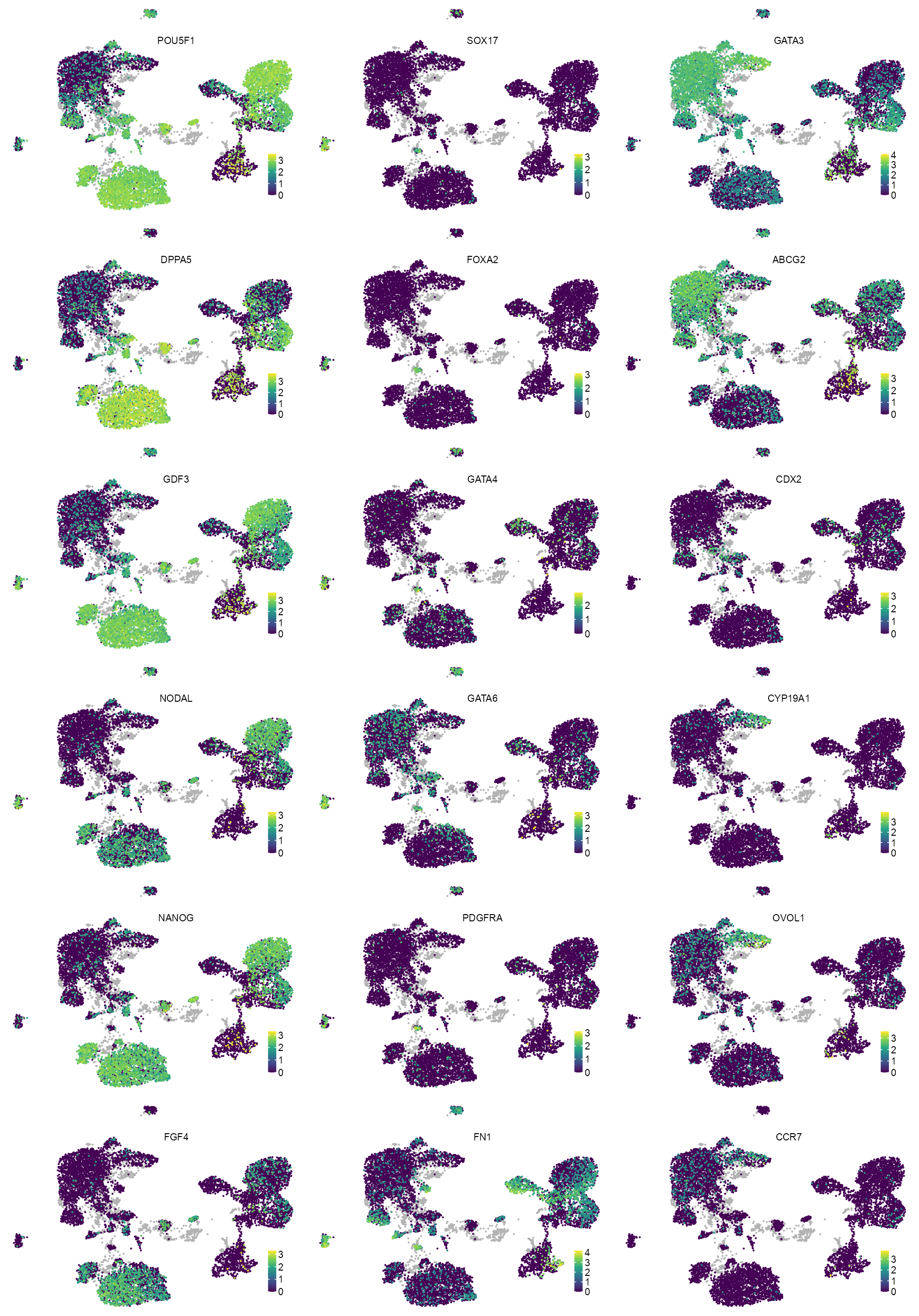
Expression
Embedding
features_selected <- c(
"ENSG00000204531_POU5F1",
"ENSG00000203909_DPPA5",
"ENSG00000184344_GDF3",
"ENSG00000156574_NODAL",
"ENSG00000111704_NANOG",
"ENSG00000075388_FGF4",
#
"ENSG00000164736_SOX17",
"ENSG00000125798_FOXA2",
"ENSG00000136574_GATA4",
"ENSG00000141448_GATA6",
"ENSG00000134853_PDGFRA",
"ENSG00000115414_FN1",
#
"ENSG00000107485_GATA3",
"ENSG00000118777_ABCG2",
"ENSG00000165556_CDX2",
"ENSG00000137869_CYP19A1",
"ENSG00000172818_OVOL1",
"ENSG00000126353_CCR7"
)
purrr::map(features_selected, \(x) {
selected_feature <- x
values <- log10(calc_cpm(matrix_readcount_use)[x, embedding$cell] + 1)
values[embedding$batch == "PRJEB11202"] <- NA
plot_embedding(
data = embedding[, c(x_column, y_column)],
color = values,
label = NULL,
color_legend = TRUE,
sort_values = TRUE,
rasterise = RASTERISED,
geom_point_size = 0.5,
na_value = "grey70"
) +
theme_customized_embedding(
x = CB_POSITION[1],
y = CB_POSITION[2],
void = TRUE,
legend_key_size = c(1.5, 1.5)
) +
ggplot2::annotate(
geom = "text",
x = x_label,
y = y_label,
label = x |> stringr::str_remove(pattern = "^E.+_"),
family = "Arial",
color = "black",
size = 5 / ggplot2::.pt,
hjust = 0.5,
vjust = 0
# parse = TRUE
)
}) |>
purrr::reduce(`+`) +
patchwork::plot_layout(ncol = 3, byrow = FALSE) +
patchwork::plot_annotation(
theme = ggplot2::theme(plot.margin = ggplot2::margin())
)
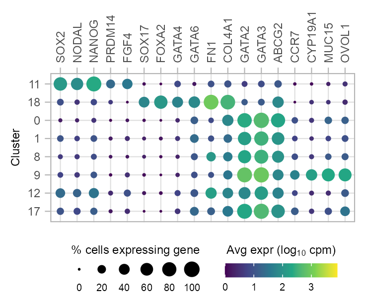
Lollipop
clusters_selected_lollipop <- c(
11,
18,
0, 1, 8, 9, 12, 17
)
cells_selected_lollipop <- purrr::map(clusters_selected_lollipop, \(x) {
embedding |>
filter(
louvain == x,
batch != "PRJEB11202"
) |>
pull(cell)
})
names(cells_selected_lollipop) <- clusters_selected_lollipop
features_selected <- c(
"ENSG00000181449_SOX2",
"ENSG00000156574_NODAL",
"ENSG00000111704_NANOG",
"ENSG00000147596_PRDM14",
"ENSG00000075388_FGF4",
#
"ENSG00000164736_SOX17",
"ENSG00000125798_FOXA2",
"ENSG00000136574_GATA4",
"ENSG00000141448_GATA6",
"ENSG00000115414_FN1",
"ENSG00000187498_COL4A1",
#
"ENSG00000179348_GATA2",
"ENSG00000107485_GATA3",
"ENSG00000118777_ABCG2",
#
"ENSG00000126353_CCR7",
"ENSG00000137869_CYP19A1",
"ENSG00000169550_MUC15",
"ENSG00000172818_OVOL1"
)
plot_lollipop(
cells = cells_selected_lollipop,
features = features_selected,
matrix_cpm = calc_cpm(matrix_readcount_use),
size_range_limits = c(0, 4),
dot_size = 3
) +
ggplot2::theme(
legend.box = "horizontal",
axis.text.x.top = ggplot2::element_text(
angle = 90, vjust = 0.5, hjust = 0
)
)
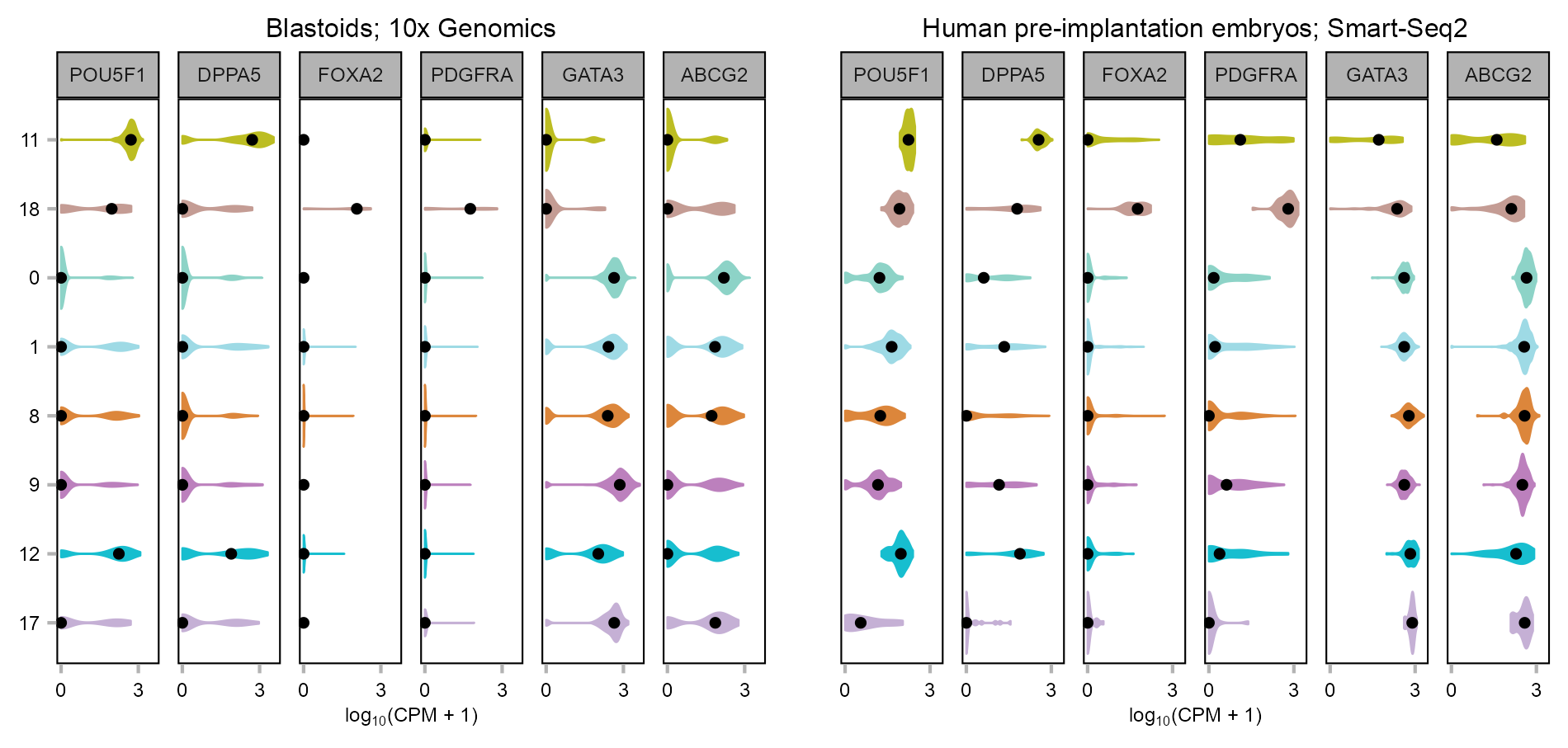
Violin
features_selected <- c(
"ENSG00000204531_POU5F1",
"ENSG00000203909_DPPA5",
"ENSG00000125798_FOXA2",
"ENSG00000134853_PDGFRA",
"ENSG00000107485_GATA3",
"ENSG00000118777_ABCG2"
)
clusters_selected_violin <- c(
11,
18,
0, 1, 8, 9, 12, 17
)
# blastoid
cells_violin <- purrr::map(clusters_selected_violin, \(x) {
embedding |>
dplyr::filter(
louvain == x,
batch != "PRJEB11202"
) |>
dplyr::pull(cell)
})
names(cells_violin) <- clusters_selected_violin
p_violin_blastoid <- plot_violin(
cells = cells_violin,
features = features_selected,
matrix_cpm = calc_cpm(matrix_readcount_use),
x_range_breaks = NULL
) +
ggplot2::scale_fill_manual(
name = NULL,
values = color_palette_cluster
) +
ggplot2::scale_color_manual(
name = NULL,
values = color_palette_cluster
) +
ggplot2::labs(title = "Blastoids; 10x Genomics") +
theme_customized_violin(panel_border_color = "black") +
ggplot2::theme(
plot.title = ggplot2::element_text(
family = "Arial",
size = 8,
margin = ggplot2::margin(
t = 0, r = 0, b = 1, l = 0,
unit = "mm"
),
hjust = 0.5
)
)Warning: Using `size` aesthetic for lines was deprecated in ggplot2 3.4.0. Please use
`linewidth` instead.
ℹ The deprecated feature was likely used in the ggplot2 package.
Please report the issue at <https://github.com/tidyverse/ggplot2/issues>.# in vivo
cells_violin <- purrr::map(clusters_selected_violin, \(x) {
embedding |>
filter(
louvain == x,
batch == "PRJEB11202"
) |>
pull(cell)
})
names(cells_violin) <- clusters_selected_violin
# re-aligned
p_violin_PRJEB11202 <- plot_violin(
cells = cells_violin,
features = features_selected,
matrix_cpm = calc_cpm(matrix_readcount_use),
x_range_breaks = NULL,
y_title = NULL
) +
ggplot2::scale_fill_manual(
name = NULL,
values = color_palette_cluster
) +
ggplot2::scale_color_manual(
name = NULL,
values = color_palette_cluster
) +
ggplot2::labs(title = "Human pre-implantation embryos; Smart-Seq2") +
theme_customized_violin(panel_border_color = "black") +
ggplot2::theme(
plot.title = ggplot2::element_text(
family = "Arial",
size = 8,
margin = ggplot2::margin(
t = 0, r = 0, b = 1, l = 0,
unit = "mm"
),
hjust = 0.5
)
)
p_violin_PRJEB11202 <- p_violin_PRJEB11202 +
theme(
axis.text.y = element_blank(),
axis.ticks.y = element_blank()
)
p_violin_blastoid_dims <- patchwork::get_dim(p_violin_blastoid)
p_violin_PRJEB11202_aligned <- patchwork::set_dim(
p_violin_PRJEB11202,
p_violin_blastoid_dims
)gridExtra::grid.arrange(
p_violin_blastoid, p_violin_PRJEB11202_aligned,
ncol = 2,
clip = FALSE
)
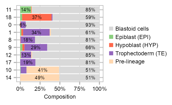
Cluster composition
clusters_selected <- c(
11,
18,
0, 1, 8, 9, 12, 17,
10, 14
)
cell_distribution_labels_right <- calc_group_composition(
data = embedding,
x = "louvain",
group = "lineage"
) |>
dplyr::filter(
is.na(lineage),
louvain %in% clusters_selected
) |>
dplyr::mutate(
louvain = factor(
louvain,
levels = rev(louvain)
)
)
cell_distribution_labels_left <- tibble::tribble(
~louvain, ~lineage, ~label_position, ~percentage,
11L, "EPI", 0.068306011, 0.136612022,
18L, "HYP", 0.20930232, 0.37209302,
0L, "TE", 0.036855838, 0.063274625,
1L, "TE", 0.20350404, 0.33513028,
8L, "TE", 0.095531587, 0.181818182,
9L, "TE", 0.19649123, 0.2877193,
12L, "TE", 0.073972603, 0.126027397,
17L, "TE", 0.09583335, 0.1916667,
10L, "Pre-lineage", 0.284146342, 0.412195122,
14L, "Pre-lineage", 0.24698795, 0.4939759
) |>
dplyr::mutate(
louvain = factor(
louvain,
levels = rev(clusters_selected)
)
)
calc_group_composition(
data = embedding,
x = "louvain",
group = "lineage"
) |>
dplyr::filter(louvain %in% clusters_selected) |>
dplyr::mutate(
louvain = factor(louvain, levels = rev(clusters_selected)),
lineage = dplyr::case_when(
is.na(lineage) ~ "Blastoid",
TRUE ~ as.character(lineage)
),
lineage = factor(lineage,
levels = rev(c("EPI", "HYP", "TE", "Pre-lineage", "Blastoid"))
)
) |>
plot_barplot(
x = "louvain",
y = "percentage",
z = "lineage"
) +
ggplot2::theme(
panel.grid.major.y = ggplot2::element_line(color = "grey80")
) +
ggplot2::coord_flip() +
ggplot2::scale_fill_manual(
name = NULL,
values = c("grey85", "#8ace7e", "#ff684c", "#9467bd", "#ffd8b1"),
breaks = c("Blastoid", "EPI", "HYP", "TE", "Pre-lineage"),
labels = c(
"Blastoid cells", "Epiblast (EPI)", "Hypoblast (HYP)",
"Trophectoderm (TE)", "Pre-lineage"
)
) +
ggplot2::geom_text(
ggplot2::aes(
y = label_position,
x = louvain,
label = scales::percent(percentage, accuracy = 1L),
group = NULL
),
size = 1.8,
family = "Arial",
color = "black",
data = cell_distribution_labels_left,
hjust = 0.5
) +
ggplot2::geom_text(
ggplot2::aes(
y = 0.825,
x = louvain,
label = scales::percent(percentage, accuracy = 1L),
group = NULL
),
size = 1.8,
family = "Arial",
color = "black",
data = cell_distribution_labels_right,
hjust = 0
)
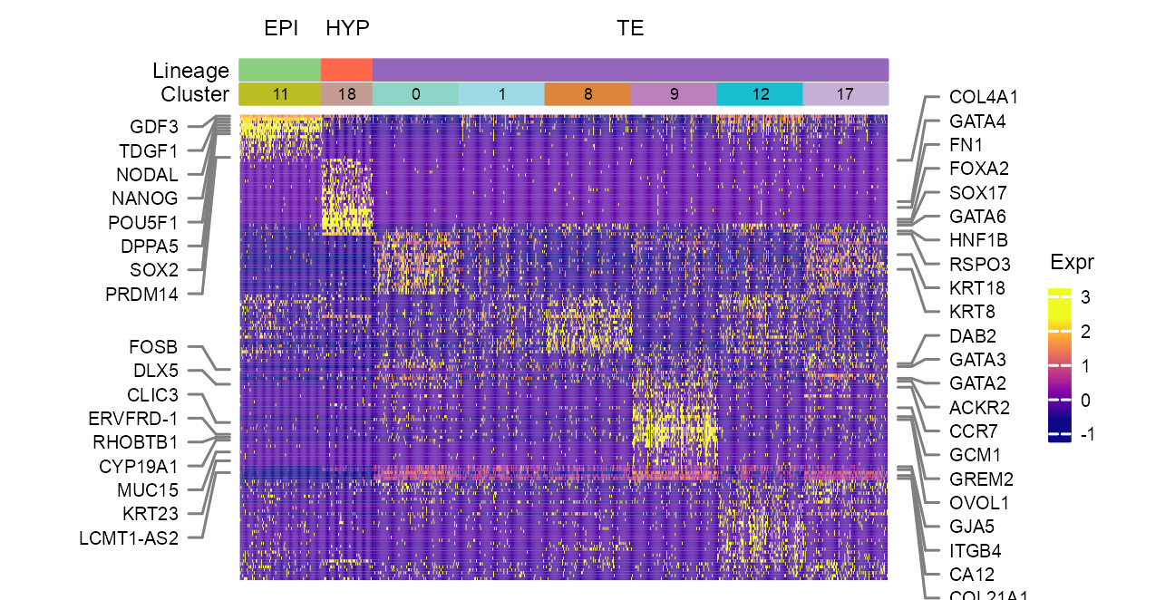
Heatmap construction
# prepare features; cells; heatmap matrix;
features_heatmap <- c(
"ENSG00000204531_POU5F1",
"ENSG00000184344_GDF3",
"ENSG00000203909_DPPA5",
"ENSG00000181449_SOX2",
"ENSG00000111704_NANOG",
"ENSG00000241186_TDGF1",
"ENSG00000156574_NODAL",
"ENSG00000254339_AC064802.1",
"ENSG00000283567_C19orf85",
"ENSG00000151650_VENTX",
"ENSG00000163032_VSNL1",
"ENSG00000159231_CBR3",
"ENSG00000145423_SFRP2",
"ENSG00000006468_ETV1",
"ENSG00000147596_PRDM14",
#
"ENSG00000136574_GATA4",
"ENSG00000164266_SPINK1",
"ENSG00000158966_CACHD1",
"ENSG00000164093_PITX2",
"ENSG00000087303_NID2",
"ENSG00000174358_SLC6A19",
"ENSG00000134962_KLB",
"ENSG00000167780_SOAT2",
"ENSG00000110245_APOC3",
"ENSG00000170558_CDH2",
"ENSG00000125848_FLRT3",
"ENSG00000129538_RNASE1",
"ENSG00000100079_LGALS2",
"ENSG00000134853_PDGFRA",
"ENSG00000164736_SOX17",
"ENSG00000017427_IGF1",
"ENSG00000275410_HNF1B",
"ENSG00000118137_APOA1",
"ENSG00000198336_MYL4",
"ENSG00000171557_FGG",
"ENSG00000125798_FOXA2",
"ENSG00000146374_RSPO3",
"ENSG00000115414_FN1",
"ENSG00000164292_RHOBTB3",
"ENSG00000141448_GATA6",
"ENSG00000187498_COL4A1",
#
"ENSG00000196549_MME",
"ENSG00000138814_PPP3CA",
"ENSG00000082074_FYB1",
"ENSG00000123191_ATP7B",
"ENSG00000175318_GRAMD2A",
"ENSG00000100593_ISM2",
"ENSG00000265107_GJA5",
"ENSG00000226887_ERVMER34-1",
"ENSG00000183734_ASCL2",
"ENSG00000143850_PLEKHA6",
"ENSG00000103534_TMC5",
"ENSG00000132470_ITGB4",
"ENSG00000180999_C1orf105",
"ENSG00000109610_SOD3",
"ENSG00000143369_ECM1",
"ENSG00000204632_HLA-G",
"ENSG00000113594_LIFR",
"ENSG00000168394_TAP1",
"ENSG00000183287_CCBE1",
"ENSG00000079393_DUSP13",
"ENSG00000121769_FABP3",
"ENSG00000182985_CADM1",
"ENSG00000164692_COL1A2",
"ENSG00000112655_PTK7",
"ENSG00000134873_CLDN10",
"ENSG00000108375_RNF43",
"ENSG00000254726_MEX3A",
"ENSG00000164120_HPGD",
"ENSG00000081026_MAGI3",
"ENSG00000120738_EGR1",
"ENSG00000108960_MMD",
"ENSG00000112137_PHACTR1",
"ENSG00000166450_PRTG",
"ENSG00000164099_PRSS12",
"ENSG00000143320_CRABP2",
"ENSG00000145681_HAPLN1",
"ENSG00000113196_HAND1",
"ENSG00000198300_PEG3",
"ENSG00000101144_BMP7",
"ENSG00000174498_IGDCC3",
"ENSG00000132005_RFX1",
"ENSG00000099814_CEP170B",
"ENSG00000101986_ABCD1",
"ENSG00000144648_ACKR2",
"ENSG00000074410_CA12",
"ENSG00000125740_FOSB",
"ENSG00000183979_NPB",
"ENSG00000214049_UCA1",
"ENSG00000153071_DAB2",
"ENSG00000126353_CCR7",
"ENSG00000105880_DLX5",
"ENSG00000124749_COL21A1",
"ENSG00000112041_TULP1",
"ENSG00000120211_INSL4",
"ENSG00000223850_MYCNUT",
"ENSG00000164707_SLC13A4",
"ENSG00000173157_ADAMTS20",
"ENSG00000196482_ESRRG",
"ENSG00000180875_GREM2",
"ENSG00000170255_MRGPRX1",
"ENSG00000267943_AC010328.1",
"ENSG00000172818_OVOL1",
"ENSG00000137270_GCM1",
"ENSG00000137869_CYP19A1",
"ENSG00000135678_CPM",
"ENSG00000171476_HOPX",
"ENSG00000249861_LGALS16",
"ENSG00000108244_KRT23",
"ENSG00000169550_MUC15",
"ENSG00000260034_LCMT1-AS2",
"ENSG00000269526_ERVV-1",
"ENSG00000028137_TNFRSF1B",
"ENSG00000124731_TREM1",
"ENSG00000072422_RHOBTB1",
"ENSG00000185215_TNFAIP2",
"ENSG00000164877_MICALL2",
"ENSG00000244476_ERVFRD-1",
"ENSG00000280109_PLAC4",
"ENSG00000111057_KRT18",
"ENSG00000170421_KRT8",
"ENSG00000169583_CLIC3",
"ENSG00000107485_GATA3",
"ENSG00000179348_GATA2",
"ENSG00000187186_AL162231.1",
"ENSG00000176155_CCDC57",
"ENSG00000133243_BTBD2",
"ENSG00000179364_PACS2",
"ENSG00000237651_C2orf74",
"ENSG00000125726_CD70",
"ENSG00000156587_UBE2L6",
"ENSG00000182165_TP53TG1",
"ENSG00000163017_ACTG2",
"ENSG00000143632_ACTA1",
"ENSG00000119632_IFI27L2",
"ENSG00000185847_LINC01405",
"ENSG00000116661_FBXO2",
"ENSG00000196878_LAMB3",
"ENSG00000122861_PLAU",
"ENSG00000142227_EMP3",
"ENSG00000011422_PLAUR",
"ENSG00000100985_MMP9",
"ENSG00000026508_CD44",
"ENSG00000104368_PLAT",
"ENSG00000164171_ITGA2",
"ENSG00000101198_NKAIN4",
"ENSG00000116774_OLFML3",
"ENSG00000125398_SOX9",
"ENSG00000124225_PMEPA1",
"ENSG00000118785_SPP1",
"ENSG00000163453_IGFBP7",
"ENSG00000182871_COL18A1",
"ENSG00000110925_CSRNP2",
"ENSG00000165886_UBTD1",
"ENSG00000115073_ACTR1B",
"ENSG00000256288_AC022075.3",
"ENSG00000228106_AL392172.1",
"ENSG00000163577_EIF5A2"
)
# heatmap matrix
clusters_selected_heatmap <- c(
11,
18,
0, 1, 8, 9, 12, 17
)
matrix_heatmap <- calc_cpm(matrix_readcount_use)[
features_heatmap,
embedding |>
dplyr::filter(
louvain %in% clusters_selected_heatmap,
batch != "PRJEB11202"
) |>
dplyr::pull(cell)
]
matrix_heatmap <- matrix_heatmap[rowSums(matrix_heatmap) != 0, ]
matrix_heatmap <- log10(matrix_heatmap + 1)
matrix_heatmap <- t(scale(t(matrix_heatmap)))
heatmap_limits <- quantile(matrix_heatmap, c(0.05, 0.95))
matrix_heatmap[matrix_heatmap < heatmap_limits[1]] <- heatmap_limits[1]
matrix_heatmap[matrix_heatmap > heatmap_limits[2]] <- heatmap_limits[2]# sample cells
cells_heatmap_sampled <- purrr::map(clusters_selected_heatmap, \(x) {
cells_in_group <- embedding |>
filter(
louvain == x,
batch != "PRJEB11202"
) |>
pull(cell)
cat(length(cells_in_group), "\n")
if (length(cells_in_group) >= 100) {
c <- sample(cells_in_group, 100)
} else {
c <- cells_in_group
}
return(c)
})
## 312
## 51
## 1428
## 682
## 528
## 376
## 310
## 97
names(cells_heatmap_sampled) <- clusters_selected_heatmap
# cells
clusters_EPI <- 11
clusters_HYP <- 18
clusters_TE <- c(0, 1, 8, 9, 12, 17)
cells_heatmap_EPI <- embedding |>
dplyr::filter(
batch != "PRJEB11202",
louvain %in% clusters_EPI,
cell %in% unlist(cells_heatmap_sampled)
) |>
dplyr::pull(cell)
cells_heatmap_HYP <- embedding |>
dplyr::filter(
batch != "PRJEB11202",
louvain %in% clusters_HYP,
cell %in% unlist(cells_heatmap_sampled)
) |>
dplyr::pull(cell)
cells_heatmap_TE <- cells_heatmap_sampled[as.character(clusters_TE)] |>
unlist()
purrr::map_int(
list(cells_heatmap_EPI, cells_heatmap_HYP, cells_heatmap_TE),
length
)
## [1] 100 51 597# features to mark
features_to_mark_left <- c(
"ENSG00000184344_GDF3",
"ENSG00000241186_TDGF1",
"ENSG00000156574_NODAL",
"ENSG00000066468_FGFR2",
"ENSG00000111704_NANOG",
"ENSG00000204531_POU5F1",
"ENSG00000203909_DPPA5",
"ENSG00000181449_SOX2",
"ENSG00000186103_ARGFX",
"ENSG00000147596_PRDM14",
"ENSG00000171872_KLF17",
"ENSG00000086548_CEACAM6",
"ENSG00000166073_GPR176",
"ENSG00000125740_FOSB",
"ENSG00000105880_DLX5",
"ENSG00000169583_CLIC3",
"ENSG00000244476_ERVFRD-1",
"ENSG00000072422_RHOBTB1",
"ENSG00000137869_CYP19A1",
"ENSG00000169550_MUC15",
"ENSG00000108244_KRT23",
"ENSG00000260034_LCMT1-AS2"
)
features_to_mark_right <- c(
"ENSG00000187498_COL4A1",
"ENSG00000136574_GATA4",
"ENSG00000115414_FN1",
"ENSG00000125798_FOXA2",
"ENSG00000164736_SOX17",
"ENSG00000141448_GATA6",
"ENSG00000275410_HNF1B",
"ENSG00000153707_PTPRD",
"ENSG00000101441_CST4",
"ENSG00000146374_RSPO3",
"ENSG00000111057_KRT18",
"ENSG00000170421_KRT8",
"ENSG00000153071_DAB2",
"ENSG00000107485_GATA3",
"ENSG00000179348_GATA2",
"ENSG00000144648_ACKR2",
"ENSG00000126353_CCR7",
"ENSG00000137270_GCM1",
"ENSG00000180875_GREM2",
"ENSG00000172818_OVOL1",
"ENSG00000265107_GJA5",
"ENSG00000132470_ITGB4",
"ENSG00000074410_CA12",
"ENSG00000124749_COL21A1"
)
#
features_to_mark_left <- features_to_mark_left[
features_to_mark_left %in% rownames(matrix_heatmap)
]
ha_left <- ComplexHeatmap::rowAnnotation(
foo = ComplexHeatmap::anno_mark(
at = which(rownames(matrix_heatmap) %in% features_to_mark_left),
labels = features_to_mark_left |>
stringr::str_remove(pattern = "E.+_"),
which = "row",
side = "left",
lines_gp = grid::gpar(col = "grey50"),
labels_gp = grid::gpar(
fontfamily = "Arial",
fontsize = 5
)
)
)
#
features_to_mark_right <- features_to_mark_right[
features_to_mark_right %in% rownames(matrix_heatmap)
]
ha_right <- ComplexHeatmap::rowAnnotation(
foo = ComplexHeatmap::anno_mark(
at = which(rownames(matrix_heatmap) %in% features_to_mark_right),
labels = features_to_mark_right |>
stringr::str_remove(pattern = "E.+_"),
which = "row",
side = "right",
lines_gp = grid::gpar(col = "grey50"),
labels_gp = grid::gpar(
fontfamily = "Arial",
fontsize = 5
)
)
)RASTERISED <- FALSE# EPI
anno_labels_tbl_EPI <- table(
ha_cluster[ha_cluster %in% clusters_EPI]
)[as.character(clusters_EPI)] |>
tibble::as_tibble() |>
dplyr::mutate(
cum_sum = cumsum(value),
position = cum_sum - value / 2
)
anno_labels_cluster_EPI <- rep(
NA, length(ha_cluster[ha_cluster %in% clusters_EPI])
)
if (nchar(as.character(clusters_EPI)) > 1) {
cluster_label <- strsplit(as.character(clusters_EPI), "")[[1]]
anno_labels_cluster_EPI[
anno_labels_tbl_EPI$position - 5
] <- cluster_label[1]
anno_labels_cluster_EPI[
anno_labels_tbl_EPI$position + 5
] <- cluster_label[2]
} else {
anno_labels_cluster_EPI[anno_labels_tbl_EPI$position] <- as.character(
clusters_EPI
)
}
ha_column_EPI <- ComplexHeatmap::HeatmapAnnotation(
#
lineage = ComplexHeatmap::anno_simple(
ha_lineage[ha_lineage == "EPI"],
# pch = anno_labels_cluster,
col = setNames(
object = c("grey85", "#8ace7e", "#ff684c", "#9467bd", "#ffd8b1"),
nm = c("Blastoid", "EPI", "HYP", "TE", "n/a")
),
which = "column",
pt_size = unit(2, "mm"),
pt_gp = grid::gpar(
fontfamily = "Arial",
fontsize = 5
),
simple_anno_size = unit(2, "mm")
),
#
cluster = ComplexHeatmap::anno_simple(
ha_cluster[ha_cluster %in% clusters_EPI],
pch = anno_labels_cluster_EPI,
col = color_palette_cluster[as.character(clusters_selected_heatmap)],
which = "column",
# pt_size = unit(2, "mm"),
pt_gp = grid::gpar(
fontfamily = "Arial",
fontsize = 5
),
simple_anno_size = unit(2, "mm")
),
#
show_annotation_name = TRUE,
annotation_label = c(
"Lineage",
"Cluster"
),
annotation_name_gp = grid::gpar(fontfamily = "Arial", fontsize = 6),
annotation_name_side = "left"
)
ht_EPI <- ComplexHeatmap::Heatmap(
matrix = matrix_heatmap[, cells_heatmap_EPI] |> as.matrix(),
rect_gp = grid::gpar(col = NA, lwd = 0),
col = col_fun,
#
row_title_gp = grid::gpar(fontfamily = "Arial", fontsize = 6),
row_title_rot = 0,
column_title_gp = grid::gpar(fontfamily = "Arial", fontsize = 6),
column_title_rot = 0,
#
cluster_rows = FALSE,
show_row_dend = FALSE,
cluster_columns = FALSE,
show_column_dend = FALSE,
#
show_row_names = FALSE,
show_column_names = FALSE,
#
top_annotation = ha_column_EPI,
bottom_annotation = NULL,
left_annotation = ha_left,
right_annotation = NULL,
#
column_split = factor(
ha_lineage[ha_lineage == "EPI"],
levels = unique(ha_lineage[ha_lineage == "EPI"])
),
column_gap = unit(0, "mm"),
#
show_heatmap_legend = FALSE,
heatmap_legend_param = list(
# title = expression(paste("Log"[10], " (CPM + 1)")),
title = "Expr",
title_gp = grid::gpar(
fontfamily = "Arial",
fontsize = 6
),
legend_direction = "vertical",
labels_gp = grid::gpar(
fontfamily = "Arial",
fontsize = 5
),
legend_height = unit(15, "mm"),
legend_width = unit(5, "mm")
),
#
use_raster = RASTERISED,
#
width = unit(8, "mm")
)
# ComplexHeatmap::draw(ht_EPI)# HYP
anno_labels_tbl_HYP <- table(
ha_cluster[ha_cluster %in% clusters_HYP]
)[as.character(clusters_HYP)] |>
as_tibble() |>
mutate(
cum_sum = cumsum(value),
position = cum_sum - value / 2
)
anno_labels_cluster_HYP <- rep(
NA, length(ha_cluster[ha_cluster %in% clusters_HYP])
)
if (nchar(as.character(clusters_HYP)) > 1) {
cluster_label <- strsplit(as.character(clusters_HYP), "")[[1]]
anno_labels_cluster_HYP[
anno_labels_tbl_HYP$position - 5
] <- cluster_label[1]
anno_labels_cluster_HYP[
anno_labels_tbl_HYP$position + 5
] <- cluster_label[2]
} else {
anno_labels_cluster_HYP[
anno_labels_tbl_HYP$position
] <- as.character(clusters_HYP)
}
ha_column_HYP <- ComplexHeatmap::HeatmapAnnotation(
#
lineage = ComplexHeatmap::anno_simple(
ha_lineage[ha_lineage == "HYP"],
# pch = anno_labels_cluster,
col = setNames(
object = c("grey85", "#8ace7e", "#ff684c", "#9467bd", "#ffd8b1"),
nm = c("Blastoid", "EPI", "HYP", "TE", "n/a")
),
which = "column",
pt_size = unit(2, "mm"),
pt_gp = grid::gpar(
fontfamily = "Arial",
fontsize = 5
),
simple_anno_size = unit(2, "mm")
),
#
cluster = ComplexHeatmap::anno_simple(
ha_cluster[ha_cluster %in% clusters_HYP],
pch = anno_labels_cluster_HYP,
col = color_palette_cluster[as.character(clusters_selected_heatmap)],
which = "column",
# pt_size = unit(2, "mm"),
pt_gp = grid::gpar(
fontfamily = "Arial",
fontsize = 5
),
simple_anno_size = unit(2, "mm")
),
#
show_annotation_name = FALSE,
annotation_label = c(
"Lineage",
"Cluster"
),
annotation_name_gp = grid::gpar(fontfamily = "Arial", fontsize = 6),
annotation_name_side = "left"
)
ht_HYP <- ComplexHeatmap::Heatmap(
matrix = matrix_heatmap[, cells_heatmap_HYP] |> as.matrix(),
rect_gp = grid::gpar(col = NA, lwd = 0),
col = col_fun,
#
row_title_gp = grid::gpar(fontfamily = "Arial", fontsize = 6),
row_title_rot = 0,
column_title_gp = grid::gpar(fontfamily = "Arial", fontsize = 6),
column_title_rot = 0,
#
cluster_rows = FALSE,
show_row_dend = FALSE,
cluster_columns = FALSE,
show_column_dend = FALSE,
#
show_row_names = FALSE,
show_column_names = FALSE,
#
top_annotation = ha_column_HYP,
bottom_annotation = NULL,
left_annotation = NULL,
right_annotation = NULL,
#
# row_split = table_s2_sheet4$ClusterID,
# row_gap = unit(0.3, "mm"),
column_split = factor(
ha_lineage[ha_lineage == "HYP"],
levels = unique(ha_lineage[ha_lineage == "HYP"])
),
column_gap = unit(0, "mm"),
#
show_heatmap_legend = FALSE,
heatmap_legend_param = list(
# title = expression(paste("Log"[10], " (CPM + 1)")),
title = "Expr",
title_gp = grid::gpar(
fontfamily = "Arial",
fontsize = 6
),
legend_direction = "vertical",
labels_gp = grid::gpar(
fontfamily = "Arial",
fontsize = 5
),
legend_height = unit(15, "mm"),
legend_width = unit(5, "mm")
),
#
use_raster = RASTERISED,
#
width = unit(5, "mm")
)
# ComplexHeatmap::draw(ht_HYP)# TE
anno_labels_tbl_TE <- table(
ha_cluster[ha_cluster %in% clusters_TE]
)[as.character(clusters_TE)] |>
tibble::enframe() |>
dplyr::mutate(
cum_sum = cumsum(value),
position = cum_sum - value / 2
)
anno_labels_tbl_TE <- purrr::map(anno_labels_tbl_TE$name, \(x) {
# works but ugly
a <- anno_labels_tbl_TE |>
filter(name == x)
if (nchar(a$name) > 1) {
cluster_label <- strsplit(as.character(a$name), "")[[1]]
a <- rbind(a, a)
a[1, 1] <- cluster_label[1]
a[2, 1] <- cluster_label[2]
a <- a |> as.data.frame()
a[1, 4] <- a[1, 4] - 5
a[2, 4] <- a[2, 4] + 5
}
return(a)
}) |>
purrr::reduce(rbind)
anno_labels_cluster_TE <- rep(
NA, length(ha_cluster[ha_cluster %in% clusters_TE])
)
anno_labels_cluster_TE[anno_labels_tbl_TE$position] <- anno_labels_tbl_TE$name
ha_column_TE <- ComplexHeatmap::HeatmapAnnotation(
#
lineage = ComplexHeatmap::anno_simple(
ha_lineage[ha_lineage == "TE"],
# pch = anno_labels_cluster,
col = setNames(
object = c("grey85", "#8ace7e", "#ff684c", "#9467bd", "#ffd8b1"),
nm = c("Blastoid", "EPI", "HYP", "TE", "n/a")
),
which = "column",
pt_size = unit(2, "mm"),
pt_gp = grid::gpar(
fontfamily = "Arial",
fontsize = 5
),
simple_anno_size = unit(2, "mm")
),
#
cluster = ComplexHeatmap::anno_simple(
ha_cluster[ha_cluster %in% clusters_TE],
pch = anno_labels_cluster_TE,
col = color_palette_cluster[as.character(clusters_selected_heatmap)],
which = "column",
# pt_size = unit(2, "mm"),
pt_gp = grid::gpar(
fontfamily = "Arial",
fontsize = 5
),
simple_anno_size = unit(2, "mm")
),
#
show_annotation_name = FALSE,
annotation_label = c(
"Lineage",
"Cluster"
),
annotation_name_gp = grid::gpar(fontfamily = "Arial", fontsize = 6),
annotation_name_side = "left"
)
ht_TE <- ComplexHeatmap::Heatmap(
matrix = matrix_heatmap[, cells_heatmap_TE] |> as.matrix(),
rect_gp = grid::gpar(col = NA, lwd = 0),
col = col_fun,
#
row_title_gp = grid::gpar(fontfamily = "Arial", fontsize = 6),
row_title_rot = 0,
column_title_gp = grid::gpar(fontfamily = "Arial", fontsize = 6),
column_title_rot = 0,
#
cluster_rows = FALSE,
show_row_dend = FALSE,
cluster_columns = FALSE,
show_column_dend = FALSE,
#
show_row_names = FALSE,
show_column_names = FALSE,
#
top_annotation = ha_column_TE,
bottom_annotation = NULL,
left_annotation = NULL,
right_annotation = ha_right,
#
column_split = factor(
ha_lineage[ha_lineage == "TE"],
levels = unique(ha_lineage[ha_lineage == "TE"])
),
column_gap = unit(0, "mm"),
#
show_heatmap_legend = FALSE,
heatmap_legend_param = list(
title = "Expr",
title_gp = grid::gpar(
fontfamily = "Arial",
fontsize = 6
),
legend_direction = "vertical",
labels_gp = grid::gpar(
fontfamily = "Arial",
fontsize = 5
),
legend_height = unit(15, "mm"),
legend_width = unit(5, "mm")
),
#
use_raster = RASTERISED,
#
width = unit(50, "mm")
)# legend
lgd_colorbar <- ComplexHeatmap::Legend(
col_fun = col_fun,
title = "Expr",
grid_height = unit(1, "mm"),
grid_width = unit(2, "mm"),
legend_height = unit(10, "mm"),
legend_width = unit(2, "mm"),
title_gp = grid::gpar(
fontfamily = "Arial",
fontsize = 6
),
labels_gp = grid::gpar(
fontfamily = "Arial",
fontsize = 5
)
)
pd <- ComplexHeatmap::packLegend(
lgd_colorbar,
# gap = unit(8, "mm"),
direction = "vertical"
)
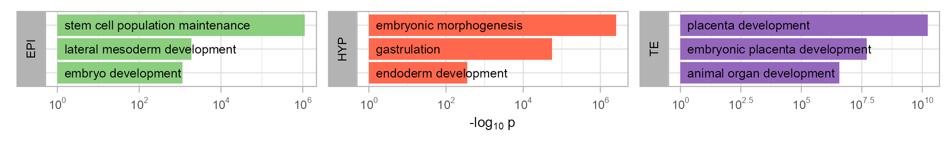
Gene Ontology enrichment
enriched_go <- tibble::tribble(
~category, ~rank, ~go_id, ~term, ~p_value, ~p_value_log,
"EPI", 1L, "GO:0019827", "stem cell population maintenance", 9e-07, 6.045757491,
"EPI", 2L, "GO:0048368", "lateral mesoderm development", 0.00053, 3.27572413,
"EPI", 3L, "GO:0009790", "embryo development", 0.00088, 3.055517328,
"HYP", 1L, "GO:0048598", "embryonic morphogenesis", 3.9e-07, 6.408935393,
"HYP", 2L, "GO:0007369", "gastrulation", 1.8e-05, 4.744727495,
"HYP", 3L, "GO:0007492", "endoderm development", 0.00284, 2.54668166,
"TE", 1L, "GO:0001890", "placenta development", 6e-11, 10.22184875,
"TE", 2L, "GO:0001892", "embryonic placenta development", 2e-08, 7.698970004,
"TE", 3L, "GO:0048513", "animal organ development", 2.7e-07, 6.568636236
)
enriched_go |>
dplyr::mutate(
category = factor(
category,
levels = c("EPI", "HYP", "TE") # |> rev()
),
rank = factor(
rank,
levels = c(3, 2, 1)
)
) |>
plot_barplot_go_enrichment(
x = p_value_log,
y = rank,
z = category
) +
ggplot2::facet_wrap(
~category,
nrow = 1,
strip.position = "left",
scales = "free_x",
labeller = ggplot2::labeller(
category = c("EPI" = "EPI", "HYP" = "HYP", "TE" = "TE")
)
) +
ggplot2::geom_text(
ggplot2::aes(
x = 0,
label = term,
group = NULL
),
size = 2.2,
family = "Arial",
color = "black",
data = enriched_go |>
dplyr::mutate(
category = factor(
category,
levels = c("EPI", "HYP", "TE")
),
rank = factor(
rank,
levels = c(3, 2, 1)
),
term = paste(" ", term)
),
hjust = 0
) +
ggplot2::scale_fill_manual(
values = c("#8ace7e", "#ff684c", "#9467bd")
)
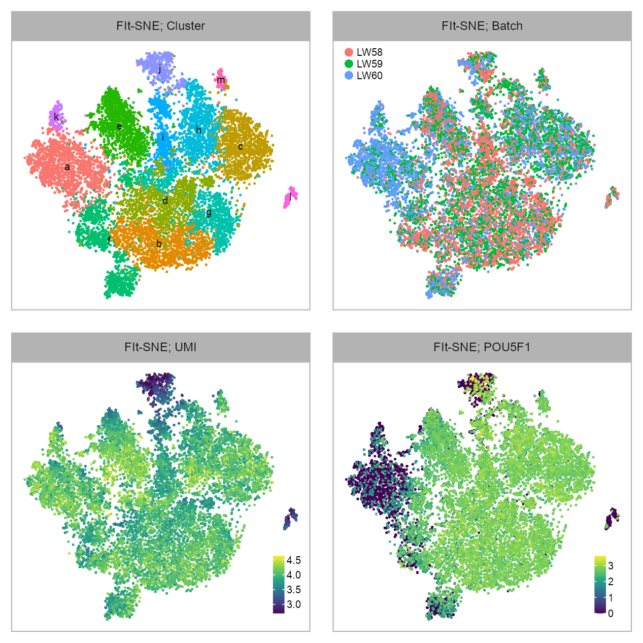
High concordance of blastoid replicates
Data loading
MATRIX_DIR <- list(
"github/data/matrices/LW36",
"github/data/matrices/LW49_LW50_LW51_LW52",
"github/data/matrices/LW58_LW59",
"github/data/matrices/LW60_LW61",
"raw/public/PRJEB11202/reformatted_matrix"
)
matrix_readcount_use <- purrr::map(MATRIX_DIR, \(x) {
load_matrix(file.path(PROJECT_DIR, x))
}) |>
purrr::reduce(cbind)
matrix_readcount_use <- matrix_readcount_use[, embedding_replicate$cell]Embedding visualization
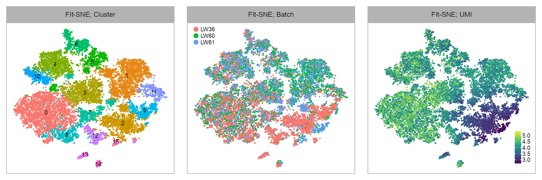
EMBEDDING_TITLE_PREFIX <- "FIt-SNE"
x_column <- "x_fitsne"
y_column <- "y_fitsne"Clustering & batch & UMI
p_embedding_replicate_louvain <- plot_embedding(
data = embedding_replicate[, c(x_column, y_column)],
color = embedding_replicate$louvain |> as.factor(),
label = glue::glue("{EMBEDDING_TITLE_PREFIX}; Cluster"),
color_labels = TRUE,
color_legend = FALSE,
sort_values = FALSE,
shuffle_values = TRUE,
rasterise = RASTERISED,
geom_point_size = GEOM_POINT_SIZE
) +
theme_customized_embedding()
p_embedding_replicate_batch <- plot_embedding(
data = embedding_replicate[, c(x_column, y_column)],
color = embedding_replicate$batch |> as.factor(),
label = glue::glue("{EMBEDDING_TITLE_PREFIX}; Batch"),
color_labels = FALSE,
color_legend = TRUE,
sort_values = FALSE,
shuffle_values = TRUE,
rasterise = RASTERISED,
geom_point_size = GEOM_POINT_SIZE
) +
theme_customized_embedding()
CB_POSITION <- c(0.875, 0.3)
p_embedding_replicate_UMI <- plot_embedding(
data = embedding_replicate[, c(x_column, y_column)],
color = log10(
Matrix::colSums(matrix_readcount_use[, embedding_replicate$cell])
),
label = glue::glue("{EMBEDDING_TITLE_PREFIX}; UMI"),
color_legend = TRUE,
sort_values = FALSE,
shuffle_values = TRUE,
rasterise = RASTERISED,
geom_point_size = GEOM_POINT_SIZE
) +
theme_customized_embedding(
x = CB_POSITION[1],
y = CB_POSITION[2]
)embedding_replicate |>
dplyr::mutate(
num_umis = colSums(matrix_readcount_use[, cell]),
num_features = colSums(matrix_readcount_use[, cell] > 0),
) |>
dplyr::group_by(batch) |>
dplyr::summarise(
num_cells = n(),
median_umis = median(num_umis),
median_features = median(num_features)
) |>
dplyr::mutate(
sample = dplyr::case_when(
batch == "LW36" ~ "Blastoid, D8; TH; 5i/L/A",
batch == "LW60" ~ "Blastoid, D9; HT; 5i/L/A",
batch == "LW61" ~ "Blastoid, D9; HT; PXGL"
)
) |>
dplyr::select(
sample, dplyr::everything()
) |>
gt::gt() |>
gt::data_color(
columns = c(median_umis),
colors = scales::col_numeric(
palette = c(
"green", "orange", "red"
),
domain = c(7500, 32000)
)
) |>
gt::summary_rows(
columns = c(sample, batch),
fns = list(
Count = ~ n()
),
decimals = 0
) |>
gt::summary_rows(
columns = c(median_umis:median_features),
fns = list(
Mean = ~ mean(.)
),
decimals = 0
) |>
gt::summary_rows(
columns = c(num_cells),
fns = list(
Sum = ~ sum(.)
),
decimals = 0
) |>
gt::tab_header(
title = gt::md("**Clustering of TH- and HT-Blastoids**; Batch")
)| Clustering of TH- and HT-Blastoids; Batch | |||||
| sample | batch | num_cells | median_umis | median_features | |
|---|---|---|---|---|---|
| Blastoid, D8; TH; 5i/L/A | LW36 | 6854 | 31193 | 5014 | |
| Blastoid, D9; HT; 5i/L/A | LW60 | 4497 | 14421 | 3337 | |
| Blastoid, D9; HT; PXGL | LW61 | 5156 | 7625 | 2185 | |
| Count | 3 | 3 | — | — | — |
| Mean | — | — | — | 17,746 | 3,512 |
| Sum | — | — | 16,507 | — | — |
purrr::reduce(
list(
p_embedding_replicate_louvain,
p_embedding_replicate_batch,
p_embedding_replicate_UMI
), `+`
) +
patchwork::plot_layout(ncol = 3) +
patchwork::plot_annotation(
theme = ggplot2::theme(plot.margin = ggplot2::margin())
)
Cluster composition
calc_group_composition(
data = embedding_replicate,
x = "louvain",
group = "batch"
) |>
dplyr::mutate(
louvain = as.factor(louvain)
) |>
plot_barplot(
x = "louvain",
y = "percentage",
z = "batch"
) +
ggplot2::guides(fill = ggplot2::guide_legend(direction = "horizontal")) +
ggplot2::theme(legend.position = "bottom")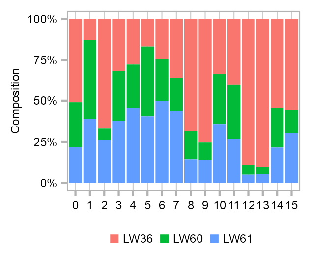
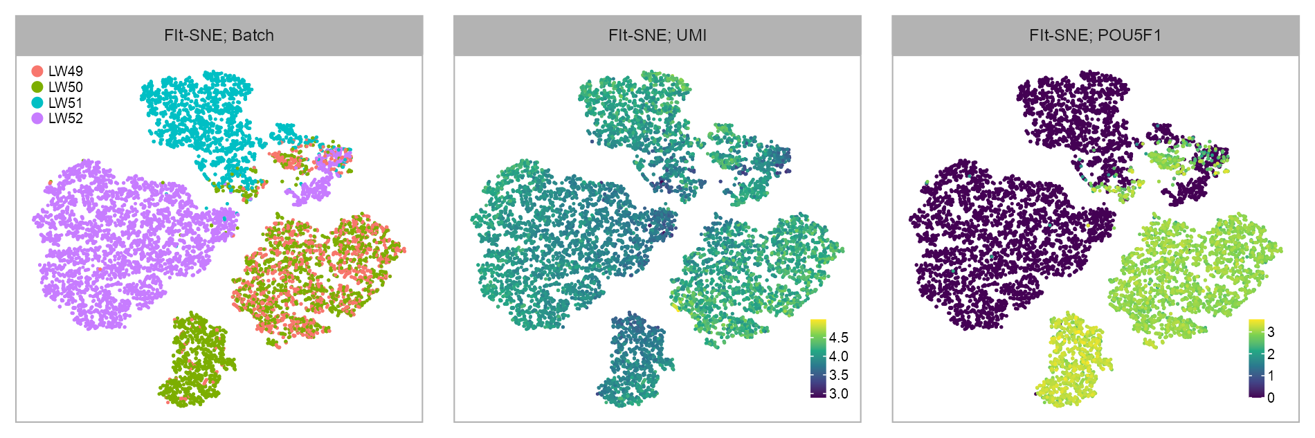
Blastoids derived stem cell lines
Data loading
MATRIX_DIR <- list(
"github/data/matrices/LW36",
"github/data/matrices/LW49_LW50_LW51_LW52",
"github/data/matrices/LW58_LW59",
"github/data/matrices/LW60_LW61",
"raw/public/PRJEB11202/reformatted_matrix"
)
matrix_readcount_use <- purrr::map(MATRIX_DIR, \(x) {
load_matrix(file.path(PROJECT_DIR, x))
}) |>
purrr::reduce(cbind)
matrix_readcount_use <- matrix_readcount_use[, embedding_stem$cell]Embedding visualization
EMBEDDING_TITLE_PREFIX <- "FIt-SNE"
x_column <- "x_fitsne"
y_column <- "y_fitsne"Clustering & batch & UMI
p_embedding_stem_batch <- plot_embedding(
data = embedding_stem[, c(x_column, y_column)],
color = embedding_stem$batch |> as.factor(),
label = glue::glue("{EMBEDDING_TITLE_PREFIX}; Batch"),
color_labels = FALSE,
color_legend = TRUE,
sort_values = FALSE,
shuffle_values = TRUE,
rasterise = RASTERISED,
geom_point_size = GEOM_POINT_SIZE
) +
theme_customized_embedding()
CB_POSITION <- c(0.875, 0.3)
p_embedding_stem_UMI <- plot_embedding(
data = embedding_stem[, c(x_column, y_column)],
color = log10(Matrix::colSums(matrix_readcount_use[, embedding_stem$cell])),
label = glue::glue("{EMBEDDING_TITLE_PREFIX}; UMI"),
color_legend = TRUE,
sort_values = FALSE,
shuffle_values = TRUE,
rasterise = RASTERISED,
geom_point_size = GEOM_POINT_SIZE
) +
theme_customized_embedding(
x = CB_POSITION[1],
y = CB_POSITION[2]
)
selected_feature <- "ENSG00000204531_POU5F1"
p_embedding_stem_POU5F1 <- plot_embedding(
data = embedding_stem[, c(x_column, y_column)],
color = log10(
calc_cpm(matrix_readcount_use[, embedding_stem$cell])
[selected_feature, ] + 1
),
label = glue::glue(
"{EMBEDDING_TITLE_PREFIX}; ",
"{selected_feature |> stringr::str_remove(pattern = \"^E.+_\")}"
),
color_legend = TRUE,
sort_values = TRUE,
rasterise = RASTERISED,
geom_point_size = GEOM_POINT_SIZE,
na_value = "grey80"
) +
theme_customized_embedding(
x = CB_POSITION[1],
y = CB_POSITION[2]
)embedding_stem |>
dplyr::mutate(
num_umis = colSums(matrix_readcount_use[, cell]),
num_features = colSums(matrix_readcount_use[, cell] > 0),
) |>
dplyr::group_by(batch) |>
dplyr::summarise(
num_cells = n(),
median_umis = median(num_umis),
median_features = median(num_features)
) |>
dplyr::mutate(
sample = dplyr::case_when(
batch == "LW49" ~ "Naïve WIRB3; 5i/L/A",
batch == "LW50" ~ "Blastoid naïve ES cells; 5i/L/A",
batch == "LW51" ~ "Blastoid nEND; NACL",
batch == "LW52" ~ "Blastoid TSCs; TSM"
)
) |>
dplyr::select(
sample, dplyr::everything()
) |>
gt::gt() |>
gt::data_color(
columns = c(median_umis),
colors = scales::col_numeric(
palette = c(
"green", "orange", "red"
),
domain = c(8500, 20000)
)
) |>
gt::summary_rows(
columns = c(sample, batch),
fns = list(
Count = ~ n()
),
decimals = 0
) |>
gt::summary_rows(
columns = c(median_umis:median_features),
fns = list(
Mean = ~ mean(.)
),
decimals = 0
) |>
gt::summary_rows(
columns = c(num_cells),
fns = list(
Sum = ~ sum(.)
),
decimals = 0
) |>
gt::tab_header(
title = gt::md("**Clustering of Blastoid Derived Cells**; Batch")
)| Clustering of Blastoid Derived Cells; Batch | |||||
| sample | batch | num_cells | median_umis | median_features | |
|---|---|---|---|---|---|
| Naïve WIRB3; 5i/L/A | LW49 | 1638 | 18363.0 | 4025.5 | |
| Blastoid naïve ES cells; 5i/L/A | LW50 | 2663 | 9022.0 | 2734.0 | |
| Blastoid nEND; NACL | LW51 | 2055 | 11767.0 | 3250.0 | |
| Blastoid TSCs; TSM | LW52 | 4486 | 8585.5 | 2581.0 | |
| Count | 4 | 4 | — | — | — |
| Mean | — | — | — | 11,934 | 3,148 |
| Sum | — | — | 10,842 | — | — |
purrr::reduce(list(
p_embedding_stem_batch,
p_embedding_stem_UMI,
p_embedding_stem_POU5F1
), `+`) +
patchwork::plot_layout(ncol = 3) +
patchwork::plot_annotation(
theme = ggplot2::theme(plot.margin = ggplot2::margin())
)
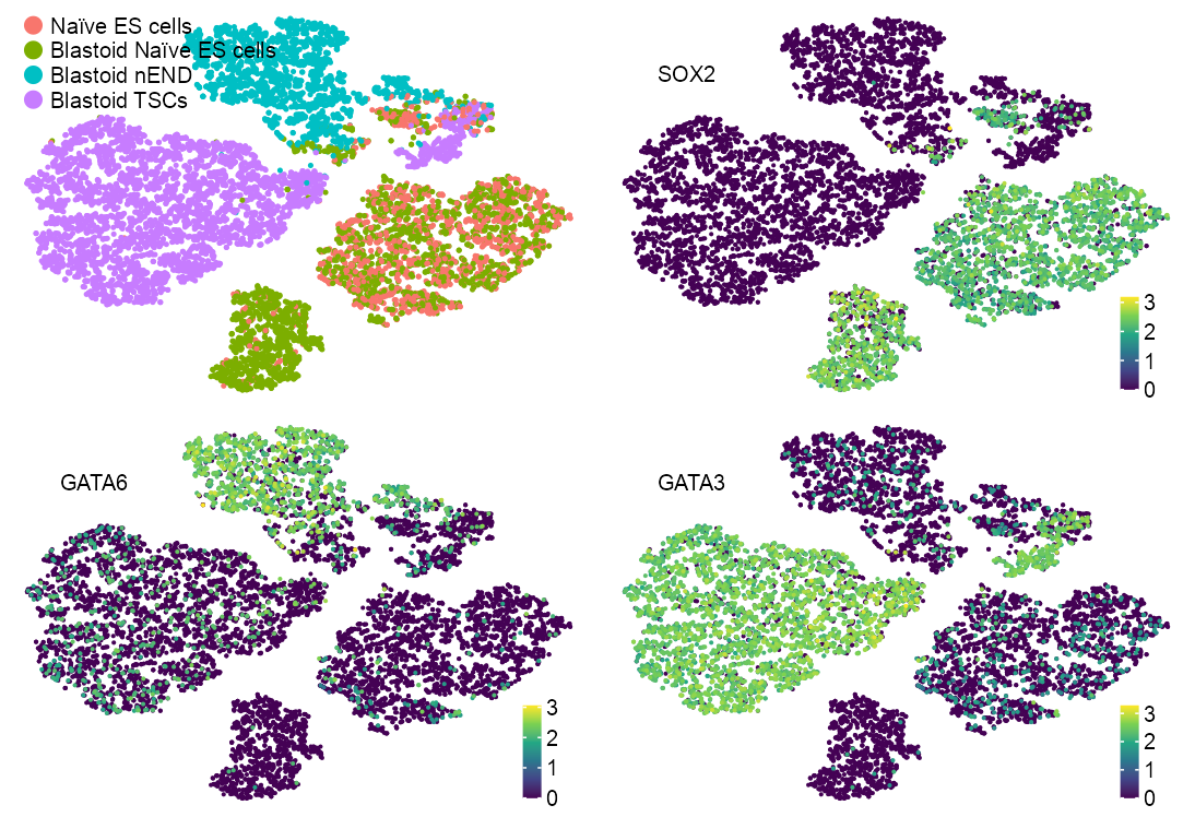
Polishing
p_embedding_stem_batch <- plot_embedding(
data = embedding_stem[, c(x_column, y_column)],
color = embedding_stem$batch |> as.factor(),
label = NULL,
color_labels = FALSE,
color_legend = TRUE,
sort_values = FALSE,
shuffle_values = TRUE,
rasterise = RASTERISED,
geom_point_size = GEOM_POINT_SIZE
) +
theme_customized_embedding(void = TRUE) +
scale_color_manual(
values = scales::hue_pal()(n = length(unique(embedding_stem$batch))),
labels = c(
"Naïve ES cells",
"Blastoid Naïve ES cells",
"Blastoid nEND",
"Blastoid TSCs"
)
)x_label <- ggplot_build(
p_embedding_stem_batch
)$layout$panel_params[[1]][c("x.range")] |>
unlist() |>
quantile(0.1)
y_label <- ggplot_build(
p_embedding_stem_batch
)$layout$panel_params[[1]][c("y.range")] |>
unlist() |>
quantile(0.8)
features_selected <- c(
"ENSG00000181449_SOX2",
"ENSG00000141448_GATA6",
"ENSG00000107485_GATA3"
)
p_embedding_stem_SOX2_GATA6_GATA3 <- purrr::map(features_selected, \(x) {
selected_feature <- x
plot_embedding(
data = embedding_stem[, c(x_column, y_column)],
color = log10(
calc_cpm(matrix_readcount_use[, embedding_stem$cell])
[selected_feature, ] + 1
),
label = NULL,
color_legend = TRUE,
sort_values = TRUE,
rasterise = RASTERISED,
geom_point_size = 0.5,
na_value = "grey80"
) +
theme_customized_embedding(
x = CB_POSITION[1],
y = CB_POSITION[2],
void = TRUE,
legend_key_size = c(1.5, 1.5)
) +
ggplot2::annotate(
geom = "text",
x = x_label,
y = y_label,
label = stringr::str_c(
x |> stringr::str_remove(pattern = "^E.+_")
),
family = "Arial",
color = "black",
size = 5 / ggplot2::.pt,
hjust = 0,
vjust = 0
# parse = TRUE
)
})list(
p_embedding_stem_batch,
p_embedding_stem_SOX2_GATA6_GATA3
) |>
purrr::reduce(`+`) +
patchwork::plot_layout(nrow = 2) +
patchwork::plot_annotation(
theme = ggplot2::theme(plot.margin = ggplot2::margin())
)
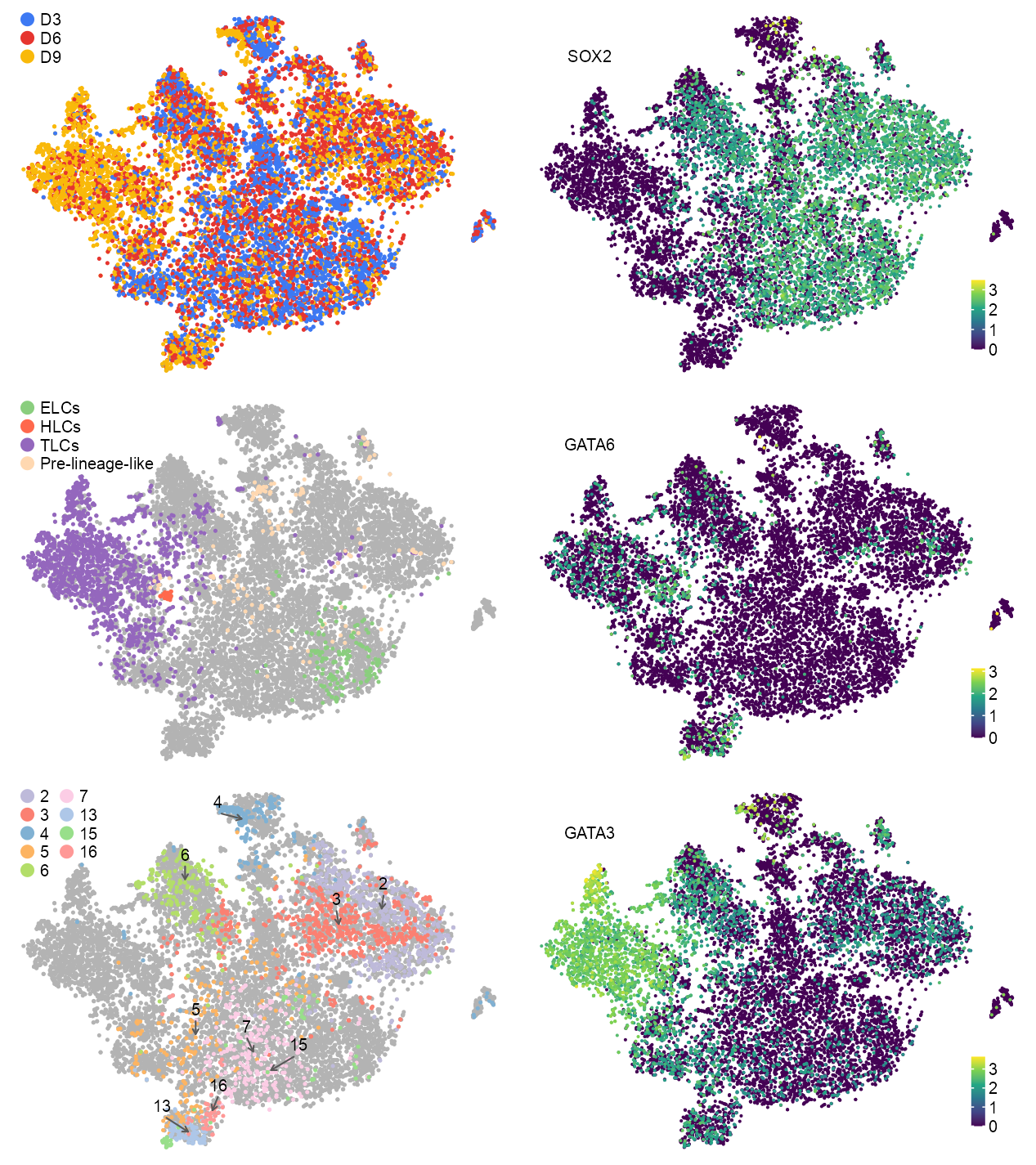
Trajectory inference
Data loading
MATRIX_DIR <- list(
"github/data/matrices/LW36",
"github/data/matrices/LW49_LW50_LW51_LW52",
"github/data/matrices/LW58_LW59",
"github/data/matrices/LW60_LW61",
"raw/public/PRJEB11202/reformatted_matrix"
)
matrix_readcount_use <- purrr::map(MATRIX_DIR, \(x) {
load_matrix(file.path(PROJECT_DIR, x))
}) |>
purrr::reduce(cbind)
matrix_readcount_use <- matrix_readcount_use[, embedding_timecourse$cell]
# clean up
rm(MATRIX_DIR)Embedding visualization
EMBEDDING_TITLE_PREFIX <- "FIt-SNE"
x_column <- "x_fitsne"
y_column <- "y_fitsne"Clustering & batch & UMI
p_embedding_timecourse_cluster <- plot_embedding(
data = embedding_timecourse[, c(x_column, y_column)],
color = letters[as.integer(embedding_timecourse$louvain + 1)] |>
as.factor(),
label = glue::glue("{EMBEDDING_TITLE_PREFIX}; Cluster"),
color_labels = TRUE,
color_legend = FALSE,
sort_values = FALSE,
shuffle_values = TRUE,
rasterise = RASTERISED,
geom_point_size = GEOM_POINT_SIZE
) +
theme_customized_embedding()
p_embedding_timecourse_batch <- plot_embedding(
data = embedding_timecourse[, c(x_column, y_column)],
color = embedding_timecourse$batch |> as.factor(),
label = glue::glue("{EMBEDDING_TITLE_PREFIX}; Batch"),
color_labels = FALSE,
color_legend = TRUE,
sort_values = FALSE,
shuffle_values = TRUE,
rasterise = RASTERISED,
geom_point_size = GEOM_POINT_SIZE
) +
theme_customized_embedding()
CB_POSITION <- c(0.875, 0.3)
p_embedding_timecourse_UMI <- plot_embedding(
data = embedding_timecourse[, c(x_column, y_column)],
color = log10(
Matrix::colSums(matrix_readcount_use[, embedding_timecourse$cell])
),
label = glue::glue("{EMBEDDING_TITLE_PREFIX}; UMI"),
color_legend = TRUE,
sort_values = FALSE,
shuffle_values = TRUE,
rasterise = RASTERISED,
geom_point_size = GEOM_POINT_SIZE
) +
theme_customized_embedding(
x = CB_POSITION[1],
y = CB_POSITION[2]
)
selected_feature <- "ENSG00000204531_POU5F1"
p_embedding_timecourse_POU5F1 <- plot_embedding(
data = embedding_timecourse[, c(x_column, y_column)],
color = log10(
calc_cpm(matrix_readcount_use[, embedding_timecourse$cell])
[selected_feature, ] + 1
),
label = glue::glue(
"{EMBEDDING_TITLE_PREFIX}; ",
"{selected_feature |> stringr::str_remove(pattern = \"^E.+_\")}"
),
color_legend = TRUE,
sort_values = TRUE,
rasterise = RASTERISED,
geom_point_size = GEOM_POINT_SIZE,
na_value = "grey80"
) +
theme_customized_embedding(
x = CB_POSITION[1],
y = CB_POSITION[2]
)list(
p_embedding_timecourse_cluster,
p_embedding_timecourse_batch,
p_embedding_timecourse_UMI,
p_embedding_timecourse_POU5F1
) |>
purrr::reduce(`+`) +
patchwork::plot_layout(ncol = 2) +
patchwork::plot_annotation(
theme = ggplot2::theme(plot.margin = ggplot2::margin())
)
Polishing
p_embedding_timecourse_batch <- plot_embedding(
data = embedding_timecourse[, c(x_column, y_column)],
color = embedding_timecourse$batch |> as.factor(),
label = NULL,
color_labels = FALSE,
color_legend = TRUE,
sort_values = FALSE,
shuffle_values = TRUE,
rasterise = RASTERISED,
geom_point_size = GEOM_POINT_SIZE
) +
theme_customized_embedding(void = TRUE) +
ggplot2::scale_color_manual(
values = yarrr::piratepal(palette = "google") |> as.character(),
labels = c("D3", "D6", "D9", "D9; PXGL")
)embedding_timecourse <- embedding_timecourse |>
dplyr::select(cell:y_fitsne) |>
dplyr::left_join(
embedding |> dplyr::select(cell, louvain_ = louvain),
by = c("cell" = "cell")
) |>
mutate(
louvain_ = case_when(
is.na(louvain_) ~ "NA",
TRUE ~ as.character(louvain_)
),
#
lineage = case_when(
louvain_ %in% c(11) ~ "EPI",
louvain_ %in% c(18) ~ "HYP",
louvain_ %in% c(0, 1, 8, 9, 12, 17) ~ "TE",
louvain_ %in% c(10, 14) ~ "Pre-lineage",
TRUE ~ "Other"
),
lineage = factor(
lineage,
levels = c("Other", "TE", "Pre-lineage", "HYP", "EPI")
),
#
cluters_selected = case_when(
louvain_ %in% c(2, 3, 4, 5, 6, 7, 13, 15, 16) ~ louvain_,
TRUE ~ "Other"
),
cluters_selected = factor(
cluters_selected,
levels = c(
"Other", "2", "3", "4", "5", "6", "7", "13", "15", "16"
)
)
)p_embedding_timecourse_lineage <- plot_embedding(
data = embedding_timecourse[, c(x_column, y_column)],
color = embedding_timecourse$lineage |> as.factor(),
label = NULL,
color_labels = FALSE,
color_legend = TRUE,
sort_values = TRUE,
shuffle_values = FALSE,
rasterise = RASTERISED,
geom_point_size = GEOM_POINT_SIZE,
na_value = "grey70"
) +
ggplot2::scale_color_manual(
name = NULL,
limits = c("TE", "Pre-lineage", "HYP", "EPI"),
values = c("grey70", "#8ace7e", "#ff684c", "#9467bd", "#ffd8b1"),
breaks = c("Other", "EPI", "HYP", "TE", "Pre-lineage"),
labels = c("Other", "ELCs", "HLCs", "TLCs", "Pre-lineage-like"),
guide = ggplot2::guides(
color = ggplot2::guide_legend(
override.aes = list(
size = 2, alpha = 1
),
ncol = 1,
reverse = TRUE,
order = 1
)
),
na.value = "grey70"
) +
theme_customized_embedding(void = TRUE)p_embedding_timecourse_cluster <- plot_embedding(
data = embedding_timecourse[, c(x_column, y_column)],
color = embedding_timecourse$cluters_selected,
label = NULL,
color_labels = FALSE,
color_legend = TRUE,
sort_values = TRUE,
shuffle_values = FALSE,
rasterise = RASTERISED,
geom_point_size = GEOM_POINT_SIZE,
geom_point_legend_ncol = 2
) +
ggplot2::scale_color_manual(
values = c("Other" = "grey70", color_palette_cluster),
limits = embedding_timecourse |>
dplyr::filter(cluters_selected != "Other") |>
dplyr::pull(cluters_selected) |>
as.character() |>
unique() |>
stringr::str_sort(numeric = TRUE),
na.value = "grey70"
) +
theme_customized_embedding(void = TRUE) +
ggrepel::geom_text_repel(
data = get_middle_points(
data = embedding_timecourse |>
dplyr::filter(cluters_selected != "Other"),
x = x_column,
y = y_column,
group = "cluters_selected"
),
ggplot2::aes(
x = x_fitsne,
y = y_fitsne,
label = cluters_selected
),
color = "black",
size = 1.8,
family = "Arial",
#
box.padding = 0.4,
point.padding = 1e-06,
min.segment.length = 0,
arrow = ggplot2::arrow(length = unit(0.015, "npc")),
max.overlaps = Inf,
nudge_x = 0,
nudge_y = 10,
#
segment.color = "grey35",
segment.size = 0.25,
segment.alpha = 1,
# segment.inflect = TRUE,
seed = 20201121
)features_selected <- c(
"ENSG00000181449_SOX2",
"ENSG00000141448_GATA6",
"ENSG00000107485_GATA3"
)
p_embedding_timecourse_SOX2_GATA6_GATA3 <- purrr::map(features_selected, \(x) {
selected_feature <- x
plot_embedding(
data = embedding_timecourse[, c(x_column, y_column)],
color = log10(
calc_cpm(matrix_readcount_use[, embedding_timecourse$cell])
[selected_feature, ] + 1
),
label = NULL,
color_legend = TRUE,
sort_values = TRUE,
rasterise = RASTERISED,
geom_point_size = 0.5,
na_value = "grey80"
) +
theme_customized_embedding(
x = CB_POSITION[1],
y = CB_POSITION[2],
void = TRUE,
legend_key_size = c(1.5, 1.5)
) +
ggplot2::annotate(
geom = "text",
x = x_label,
y = y_label,
label = stringr::str_c(
x |> stringr::str_remove(pattern = "^E.+_")
),
family = "Arial",
color = "black",
size = 5 / ggplot2::.pt,
hjust = 0.5,
vjust = 0
# parse = TRUE
)
})c(
list(
p_embedding_timecourse_batch,
p_embedding_timecourse_lineage,
p_embedding_timecourse_cluster
),
p_embedding_timecourse_SOX2_GATA6_GATA3
) |>
purrr::reduce(`+`) +
patchwork::plot_layout(ncol = 2, byrow = FALSE) +
patchwork::plot_annotation(
theme = theme(plot.margin = margin())
)
Cluster composition
calc_group_composition(
data = embedding_timecourse,
x = "louvain",
group = "batch"
) |>
dplyr::mutate(
louvain = as.factor(louvain)
) |>
plot_barplot(
x = "louvain",
y = "percentage",
z = "batch"
) +
ggplot2::scale_fill_manual(
values = yarrr::piratepal(palette = "google") %>% as.character(),
labels = c("D3", "D6", "D9", "D9; PXGL")
) +
ggplot2::guides(fill = ggplot2::guide_legend(direction = "horizontal")) +
ggplot2::theme(legend.position = "bottom")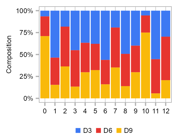
R session info
devtools::session_info()─ Session info ───────────────────────────────────────────────────────────────
setting value
version R version 4.2.1 (2022-06-23)
os macOS Monterey 12.6
system aarch64, darwin21.6.0
ui unknown
language (EN)
collate en_US.UTF-8
ctype en_US.UTF-8
tz America/Chicago
date 2022-09-25
pandoc 2.19.2 @ /opt/homebrew/bin/ (via rmarkdown)
─ Packages ───────────────────────────────────────────────────────────────────
package * version date (UTC) lib source
BayesFactor 0.9.12-4.4 2022-07-05 [1] CRAN (R 4.2.1)
BiocGenerics 0.42.0 2022-04-26 [1] Bioconductor
bit 4.0.4 2020-08-04 [1] CRAN (R 4.2.0)
bit64 4.0.5 2020-08-30 [1] CRAN (R 4.2.0)
cachem 1.0.6 2021-08-19 [1] CRAN (R 4.2.0)
Cairo 1.6-0 2022-07-05 [1] CRAN (R 4.2.1)
callr 3.7.2 2022-08-22 [1] CRAN (R 4.2.1)
circlize 0.4.15 2022-05-10 [1] CRAN (R 4.2.0)
cli 3.4.1 2022-09-23 [1] CRAN (R 4.2.1)
clue 0.3-61 2022-05-30 [1] CRAN (R 4.2.0)
cluster 2.1.4 2022-08-22 [2] CRAN (R 4.2.1)
coda 0.19-4 2020-09-30 [1] CRAN (R 4.2.0)
codetools 0.2-18 2020-11-04 [2] CRAN (R 4.2.1)
colorspace 2.0-3 2022-02-21 [1] CRAN (R 4.2.0)
commonmark 1.8.0 2022-03-09 [1] CRAN (R 4.2.0)
ComplexHeatmap 2.12.1 2022-08-09 [1] Bioconductor
crayon 1.5.1 2022-03-26 [1] CRAN (R 4.2.0)
devtools 2.4.4.9000 2022-09-23 [1] Github (r-lib/devtools@9e2793a)
digest 0.6.29 2021-12-01 [1] CRAN (R 4.2.0)
doParallel 1.0.17 2022-02-07 [1] CRAN (R 4.2.0)
dplyr * 1.0.99.9000 2022-09-23 [1] Github (tidyverse/dplyr@19c2be3)
ellipsis 0.3.2 2021-04-29 [1] CRAN (R 4.2.0)
evaluate 0.16 2022-08-09 [1] CRAN (R 4.2.1)
extrafont * 0.18 2022-04-12 [1] CRAN (R 4.2.0)
extrafontdb 1.0 2012-06-11 [1] CRAN (R 4.2.0)
fansi 1.0.3 2022-03-24 [1] CRAN (R 4.2.0)
farver 2.1.1 2022-07-06 [1] CRAN (R 4.2.1)
fastmap 1.1.0 2021-01-25 [1] CRAN (R 4.2.0)
forcats * 0.5.2.9000 2022-08-20 [1] Github (tidyverse/forcats@bd319e0)
foreach 1.5.2 2022-02-02 [1] CRAN (R 4.2.0)
fs 1.5.2.9000 2022-08-24 [1] Github (r-lib/fs@238032f)
generics 0.1.3 2022-07-05 [1] CRAN (R 4.2.1)
GetoptLong 1.0.5 2020-12-15 [1] CRAN (R 4.2.0)
ggplot2 * 3.3.6.9000 2022-09-12 [1] Github (tidyverse/ggplot2@a58b48c)
ggrepel 0.9.1 2021-01-15 [1] CRAN (R 4.2.0)
ggthemes 4.2.4 2021-01-20 [1] CRAN (R 4.2.0)
GlobalOptions 0.1.2 2020-06-10 [1] CRAN (R 4.2.0)
glue 1.6.2.9000 2022-04-22 [1] Github (tidyverse/glue@d47d6c7)
gridExtra 2.3 2017-09-09 [1] CRAN (R 4.2.0)
gt 0.7.0.9000 2022-09-23 [1] Github (rstudio/gt@4030fb7)
gtable 0.3.1.9000 2022-09-01 [1] Github (r-lib/gtable@c1a7a81)
hms 1.1.2 2022-08-19 [1] CRAN (R 4.2.1)
htmltools 0.5.3 2022-07-18 [1] CRAN (R 4.2.1)
htmlwidgets 1.5.4 2022-08-23 [1] Github (ramnathv/htmlwidgets@400cf1a)
httpuv 1.6.6 2022-09-08 [1] CRAN (R 4.2.1)
IRanges 2.30.1 2022-08-18 [1] Bioconductor
iterators 1.0.14 2022-02-05 [1] CRAN (R 4.2.0)
jpeg 0.1-9 2021-07-24 [1] CRAN (R 4.2.0)
jsonlite 1.8.0 2022-02-22 [1] CRAN (R 4.2.0)
knitr 1.40 2022-08-24 [1] CRAN (R 4.2.1)
labeling 0.4.2 2020-10-20 [1] CRAN (R 4.2.0)
later 1.3.0 2021-08-18 [1] CRAN (R 4.2.0)
lattice 0.20-45 2021-09-22 [2] CRAN (R 4.2.1)
lifecycle 1.0.2.9000 2022-09-23 [1] Github (r-lib/lifecycle@0a6860a)
lubridate * 1.8.0.9000 2022-05-24 [1] Github (tidyverse/lubridate@0bb49b2)
magick 2.7.3 2021-08-18 [1] CRAN (R 4.2.0)
magrittr 2.0.3 2022-03-30 [1] CRAN (R 4.2.0)
Matrix * 1.5-1 2022-09-13 [1] CRAN (R 4.2.1)
MatrixModels 0.5-1 2022-09-11 [1] CRAN (R 4.2.1)
matrixStats 0.62.0 2022-04-19 [1] CRAN (R 4.2.0)
memoise 2.0.1 2021-11-26 [1] CRAN (R 4.2.0)
mime 0.12 2021-09-28 [1] CRAN (R 4.2.0)
miniUI 0.1.1.1 2018-05-18 [1] CRAN (R 4.2.0)
munsell 0.5.0 2018-06-12 [1] CRAN (R 4.2.0)
mvtnorm 1.1-3 2021-10-08 [1] CRAN (R 4.2.1)
patchwork * 1.1.2.9000 2022-08-20 [1] Github (thomasp85/patchwork@c14c960)
pbapply 1.5-0 2021-09-16 [1] CRAN (R 4.2.0)
pillar 1.8.1 2022-08-19 [1] CRAN (R 4.2.1)
pkgbuild 1.3.1 2021-12-20 [1] CRAN (R 4.2.0)
pkgconfig 2.0.3 2019-09-22 [1] CRAN (R 4.2.0)
pkgload 1.3.0 2022-06-27 [1] CRAN (R 4.2.1)
png 0.1-7 2013-12-03 [1] CRAN (R 4.2.0)
prettyunits 1.1.1.9000 2022-04-22 [1] Github (r-lib/prettyunits@8706d89)
processx 3.7.0 2022-07-07 [1] CRAN (R 4.2.1)
profvis 0.3.7 2020-11-02 [1] CRAN (R 4.2.0)
promises 1.2.0.1 2021-02-11 [1] CRAN (R 4.2.0)
ps 1.7.1 2022-06-18 [1] CRAN (R 4.2.0)
purrr * 0.9000.0.9000 2022-09-24 [1] Github (tidyverse/purrr@4ab13f5)
R.cache 0.16.0 2022-07-21 [1] CRAN (R 4.2.1)
R.methodsS3 1.8.2 2022-06-13 [1] CRAN (R 4.2.0)
R.oo 1.25.0 2022-06-12 [1] CRAN (R 4.2.0)
R.utils 2.12.0 2022-06-28 [1] CRAN (R 4.2.1)
R6 2.5.1.9000 2022-08-04 [1] Github (r-lib/R6@87d5e45)
ragg 1.2.2.9000 2022-09-12 [1] Github (r-lib/ragg@904e145)
RColorBrewer 1.1-3 2022-04-03 [1] CRAN (R 4.2.0)
Rcpp 1.0.9 2022-07-08 [1] CRAN (R 4.2.1)
readr * 2.1.2.9000 2022-09-20 [1] Github (tidyverse/readr@5cac6ed)
remotes 2.4.2 2022-09-12 [1] Github (r-lib/remotes@bc0949d)
reticulate 1.26 2022-08-31 [1] CRAN (R 4.2.1)
rjson 0.2.21 2022-01-09 [1] CRAN (R 4.2.0)
rlang 1.0.6 2022-09-24 [1] Github (r-lib/rlang@66454bd)
rmarkdown 2.16.1 2022-09-24 [1] Github (rstudio/rmarkdown@9577707)
Rttf2pt1 1.3.10 2022-02-07 [1] CRAN (R 4.2.0)
S4Vectors 0.34.0 2022-04-26 [1] Bioconductor
sass 0.4.2 2022-07-16 [1] CRAN (R 4.2.1)
scales 1.2.1.9000 2022-08-20 [1] Github (r-lib/scales@b3df2fb)
sessioninfo 1.2.2 2021-12-06 [1] CRAN (R 4.2.0)
shape 1.4.6 2021-05-19 [1] CRAN (R 4.2.0)
shiny 1.7.2 2022-07-19 [1] CRAN (R 4.2.1)
stringi 1.7.8 2022-07-11 [1] CRAN (R 4.2.1)
stringr * 1.4.1.9000 2022-08-21 [1] Github (tidyverse/stringr@792bc92)
styler * 1.7.0.9002 2022-09-21 [1] Github (r-lib/styler@1f4437b)
systemfonts 1.0.4 2022-02-11 [1] CRAN (R 4.2.0)
textshaping 0.3.6 2021-10-13 [1] CRAN (R 4.2.0)
tibble * 3.1.8.9002 2022-09-24 [1] Github (tidyverse/tibble@e9db4f4)
tidyr * 1.2.1.9000 2022-09-09 [1] Github (tidyverse/tidyr@653def2)
tidyselect 1.1.2.9000 2022-09-21 [1] Github (r-lib/tidyselect@edd0a3b)
tidyverse * 1.3.2.9000 2022-09-12 [1] Github (tidyverse/tidyverse@3be8283)
tzdb 0.3.0 2022-03-28 [1] CRAN (R 4.2.0)
urlchecker 1.0.1 2021-11-30 [1] CRAN (R 4.2.0)
usethis 2.1.6.9000 2022-09-23 [1] Github (r-lib/usethis@8ecb7ab)
utf8 1.2.2 2021-07-24 [1] CRAN (R 4.2.0)
vctrs 0.4.1.9000 2022-09-19 [1] Github (r-lib/vctrs@0a219ba)
viridis 0.6.2 2021-10-13 [1] CRAN (R 4.2.0)
viridisLite 0.4.1 2022-08-22 [1] CRAN (R 4.2.1)
vroom 1.5.7.9000 2022-09-09 [1] Github (r-lib/vroom@0c2423e)
withr 2.5.0 2022-03-03 [1] CRAN (R 4.2.0)
xfun 0.33 2022-09-12 [1] CRAN (R 4.2.1)
xtable 1.8-4 2019-04-21 [1] CRAN (R 4.2.0)
yaml 2.3.5 2022-02-21 [1] CRAN (R 4.2.0)
yarrr 0.1.6 2022-04-22 [1] Github (ndphillips/yarrr@e2e4488)
[1] /opt/homebrew/lib/R/4.2/site-library
[2] /opt/homebrew/Cellar/r/4.2.1_4/lib/R/library
─ Python configuration ───────────────────────────────────────────────────────
python:         /Users/jialei/.pyenv/shims/python
libpython:      /Users/jialei/.pyenv/versions/mambaforge-4.10.3-10/lib/libpython3.9.dylib
pythonhome:     /Users/jialei/.pyenv/versions/mambaforge-4.10.3-10:/Users/jialei/.pyenv/versions/mambaforge-4.10.3-10
version:        3.9.13 | packaged by conda-forge | (main, May 27 2022, 17:00:33)  [Clang 13.0.1 ]
numpy:          /Users/jialei/.pyenv/versions/mambaforge-4.10.3-10/lib/python3.9/site-packages/numpy
numpy_version:  1.22.4
numpy:          /Users/jialei/.pyenv/versions/mambaforge-4.10.3-10/lib/python3.9/site-packages/numpy

NOTE: Python version was forced by RETICULATE_PYTHON
──────────────────────────────────────────────────────────────────────────────Citation
BibTeX citation:
@article{yu,
  author = {Leqian Yu and Yulei Wei and Jialei Duan and Daniel A.
    Schmitz and Masahiro Sakurai and Lei Wang and Kunhua Wang and Shuhua
    Zhao and Gary C. Hon and Jun Wu},
  editor = {},
  publisher = {Nature Publishing Group},
  title = {Blastocyst-Like Structures Generated from Human Pluripotent
    Stem Cells},
  journal = {Nature},
  volume = {591},
  number = {7851},
  pages = {620 - 626},
  date = {},
  url = {https://doi.org/10.1038/s41586-021-03356-y},
  doi = {10.1038/s41586-021-03356-y},
  langid = {en},
  abstract = {Human blastoids provide a readily accessible, scalable,
    versatile and perturbable alternative to blastocysts for studying
    early human development, understanding early pregnancy loss and
    gaining insights into early developmental defects.}
}
For attribution, please cite this work as:
Leqian Yu, Yulei Wei, Jialei Duan, Daniel A. Schmitz, Masahiro Sakurai,
Lei Wang, Kunhua Wang, Shuhua Zhao, Gary C. Hon, and Jun Wu. n.d.
“Blastocyst-Like Structures Generated from Human Pluripotent Stem
Cells.” Nature 591 (7851): 620–26. https://doi.org/10.1038/s41586-021-03356-y.