Blastoids Are Capable of Recapitulating Human Embryo Implantation Events

Jialei Duan

Blastoids Are Capable of Recapitulating Human Embryo Implantation Events

Author

Affiliation

Jialei Duan

UT Southwestern Medical Center

Published

Sun Sep 10, 2023 03:27:56-05:00

Sys.time()

[1] "2023-09-10 03:27:17 CDT"

Sys.timezone()

[1] "America/Chicago"

Preparation

PROJECT_DIR <- file.path(
    "/Users/jialei/Dropbox/Data/Projects/UTSW/Peri-implantation"
)

Functions

Load required packages.

library(tidyverse)
## ── Attaching core tidyverse packages ─────────────────── tidyverse 2.0.0.9000 ──
## ✔ dplyr     1.1.3          ✔ readr     2.1.4.9000
## ✔ forcats   1.0.0.9000     ✔ stringr   1.5.0.9000
## ✔ ggplot2   3.4.3.9000     ✔ tibble    3.2.1.9005
## ✔ lubridate 1.9.2.9000     ✔ tidyr     1.3.0.9000
## ✔ purrr     1.0.2.9000     
## ── Conflicts ────────────────────────────────────────── tidyverse_conflicts() ──
## ✖ dplyr::filter() masks stats::filter()
## ✖ dplyr::lag()    masks stats::lag()
## ℹ Use the conflicted package (<http://conflicted.r-lib.org/>) to force all conflicts to become errors
library(Matrix)
## 
## Attaching package: 'Matrix'
## 
## The following objects are masked from 'package:tidyr':
## 
##     expand, pack, unpack
library(patchwork)
library(extrafont)
## Registering fonts with R

source(file = file.path(SCRIPT_DIR, "utilities.R"))

`%+replace%` <- ggplot2::`%+replace%`

add_panel_border <- function() {
    ggplot2::theme(
        plot.background = element_rect(
            colour = "grey70", fill = NA, linewidth = 0.25
        )
    )
}

theme_customized_clear <- function() {
    ggplot2::theme(
        legend.background = ggplot2::element_blank(),
        panel.background = ggplot2::element_blank(),
        panel.grid.major = ggplot2::element_blank(),
        panel.grid.minor = ggplot2::element_blank(),
        #
        plot.background = ggplot2::element_blank(),
        # plot.background = element_rect(
        #     colour = "grey70", fill = NA, linewidth = 0.25
        # ),
        #
        # axis.ticks.length = ggplot2::unit(0, "pt"),
        panel.border = ggplot2::element_blank(),
        plot.margin = ggplot2::unit(c(0, 0, 0, 0), "lines")
    )
}

Python env

np <- reticulate::import("numpy", convert = TRUE)
# scipy.sparse <- reticulate::import(module = "scipy.sparse", convert = TRUE)
cat("numpy version:", np$`__version__`, "\n")

numpy version: 1.24.3

ad <- reticulate::import(module = "anndata", convert = TRUE)
print(ad$`__version__`)

[1] "0.8.0"

reticulate::py_config()

python:         /Users/jialei/.pyenv/shims/python
libpython:      /Users/jialei/.pyenv/versions/mambaforge-22.9.0-3/lib/libpython3.10.dylib
pythonhome:     /Users/jialei/.pyenv/versions/mambaforge-22.9.0-3:/Users/jialei/.pyenv/versions/mambaforge-22.9.0-3
version:        3.10.9 | packaged by conda-forge | (main, Feb  2 2023, 20:26:08) [Clang 14.0.6 ]
numpy:          /Users/jialei/.pyenv/versions/mambaforge-22.9.0-3/lib/python3.10/site-packages/numpy
numpy_version:  1.24.3
numpy:          /Users/jialei/.pyenv/versions/mambaforge-22.9.0-3/lib/python3.10/site-packages/numpy

NOTE: Python version was forced by RETICULATE_PYTHON

Embedding

embedding <- vroom::vroom(
    file = file.path(
        PROJECT_DIR,
        "clustering",
        "LW186_LW187_LW188_LW189_LW202_LW203_LW204",
        "exploring",
        CLUSTERING_METHOD,
        EMBEDDING_FILE
    ),
    show_col_types = FALSE
) |>
    dplyr::mutate(
        batch = dplyr::case_when(
            batch == "GSM4734573" ~ "PRJNA658478",
            TRUE ~ batch
        ),
        bioproject = dplyr::case_when(
            batch %in% c("LW60", "LW61") ~ "PRJNA632839",
            #
            batch %in% c("GSM3956280", "GSM3956281") ~ "PRJNA555602",
            batch %in% c("GSM4734573") ~ "PRJNA658478",
            #
            batch %in% c(
                "GSM4816780", "GSM4816781", "GSM4816782"
            ) ~ "PRJNA667174",
            batch %in% c("GSM5387817", "GSM5387818") ~ "PRJNA738498",
            TRUE ~ batch
        )
    )

embedding_stromal <- vroom::vroom(
    file = file.path(
        PROJECT_DIR,
        "clustering",
        "LW186_LW187_LW188_LW189_LW202_LW203_LW204_stromal",
        "exploring",
        "Scanpy_Harmony_variable",
        "embedding_ncomponents16_seed20210719.csv.gz"
    ),
    show_col_types = FALSE
) |>
    dplyr::mutate(
        batch_annotated = dplyr::case_when(
            batch %in% c("LW187", "LW189") ~ "Blastocyst (fibronectin)",
            batch %in% c("LW186", "LW188") ~ "Blastocyst (stromal cells)",
            batch %in% c("LW202") ~ "Blastoid (fibronectin)",
            batch %in% c("LW203") ~ "Stromal cells",
            batch %in% c("LW204") ~ "Blastoid (stromal cells)"
        )
    )

Matrix

adata_files <- c(
    purrr::map(
        c("LW186", "LW187", "LW188", "LW189", "LW202", "LW203", "LW204"), \(x) {
            file.path(
                PROJECT_DIR,
                "raw",
                x,
                "matrix",
                "adata.h5ad"
            )
        }
    )
)

adata_files <- unique(adata_files)
purrr::map_lgl(adata_files, file.exists)

[1] TRUE TRUE TRUE TRUE TRUE TRUE TRUE

BACKED <- NULL
matrix_readcount_use <- purrr::map(adata_files, \(x) {
    cat(x, "\n")
    ad$read_h5ad(
        filename = x, backed = BACKED
    ) |>
        extract_matrix_from_adata(cells_selected = embedding$cell)
}) |>
    purrr::reduce(cbind)

/Users/jialei/Dropbox/Data/Projects/UTSW/Peri-implantation/raw/LW186/matrix/adata.h5ad 
/Users/jialei/Dropbox/Data/Projects/UTSW/Peri-implantation/raw/LW187/matrix/adata.h5ad 
/Users/jialei/Dropbox/Data/Projects/UTSW/Peri-implantation/raw/LW188/matrix/adata.h5ad 
/Users/jialei/Dropbox/Data/Projects/UTSW/Peri-implantation/raw/LW189/matrix/adata.h5ad 
/Users/jialei/Dropbox/Data/Projects/UTSW/Peri-implantation/raw/LW202/matrix/adata.h5ad 
/Users/jialei/Dropbox/Data/Projects/UTSW/Peri-implantation/raw/LW203/matrix/adata.h5ad 
/Users/jialei/Dropbox/Data/Projects/UTSW/Peri-implantation/raw/LW204/matrix/adata.h5ad

matrix_readcount_use <- matrix_readcount_use[
    , sort(colnames(matrix_readcount_use))
]
matrix_readcount_use |> dim()

[1] 33538 39755

# sanity check
stopifnot(
    ncol(matrix_readcount_use) == nrow(embedding)
)

Metadata

BACKED <- "r"
cell_metadata <- purrr::map(adata_files, \(x) {
    ad$read_h5ad(
        filename = x, backed = BACKED
    )$obs |>
        tibble::rownames_to_column(var = "cell") |>
        dplyr::select(cell, everything())
}) |>
    dplyr::bind_rows()

embedding |>
    dplyr::left_join(
        cell_metadata |>
            dplyr::select(cell, num_umis),
        by = "cell"
    ) |>
    dplyr::group_by(batch) |>
    dplyr::summarise(
        num_cells = n(),
        meidan_umis = median(num_umis)
    ) |>
    gt::gt()

batch	num_cells	meidan_umis
LW186	10977	3026
LW187	3690	4980
LW188	6838	3738
LW189	3250	5344
LW202	4833	3834
LW203	2571	5254
LW204	7596	2405

Check memory usage.

walk(list(matrix_readcount_use, embedding), \(x) {
    print(object.size(x), units = "auto", standard = "SI")
})

818.1 MB
8.6 MB

Blastoids resemble human embryo implantation

Inspection

embedding |>
    dplyr::left_join(
        cell_metadata |> dplyr::select(cell, num_umis),
        by = "cell"
    ) |>
    dplyr::group_by(batch) |>
    dplyr::summarise(
        num_cells = n(),
        median_umis = median(num_umis)
    ) |>
    gt::gt() |>
    gt::data_color(
        columns = c(median_umis),
        fn = scales::col_numeric(
            palette = c(
                "green", "orange", "red"
            ),
            domain = NULL
        )
    ) |>
    gt::fmt_number(
        columns = c(median_umis),
        sep_mark = ",",
        decimals = 1,
        use_seps = TRUE,
        suffixing = FALSE
    ) |>
    gt::fmt_number(
        columns = c(num_cells),
        sep_mark = ",",
        decimals = 0,
        use_seps = TRUE,
        suffixing = FALSE
    ) |>
    gt::grand_summary_rows(
        columns = c(num_cells),
        fns = list(
            Sum = ~ sum(.)
        ),
        fmt = ~ gt::fmt_number(., decimals = 0, use_seps = TRUE)
    )

	batch	num_cells	median_umis
	LW186	10,977	3,026.0
	LW187	3,690	4,980.0
	LW188	6,838	3,738.0
	LW189	3,250	5,344.0
	LW202	4,833	3,834.0
	LW203	2,571	5,254.0
	LW204	7,596	2,405.0
Sum	—	39,755	—

GEOM_POINT_SIZE <- 0.25
RASTERISED <- TRUE
x_column <- "x_umap_min_dist=0.1"
y_column <- "y_umap_min_dist=0.1"

EMBEDDING_TITLE_PREFIX <- "UMAP"
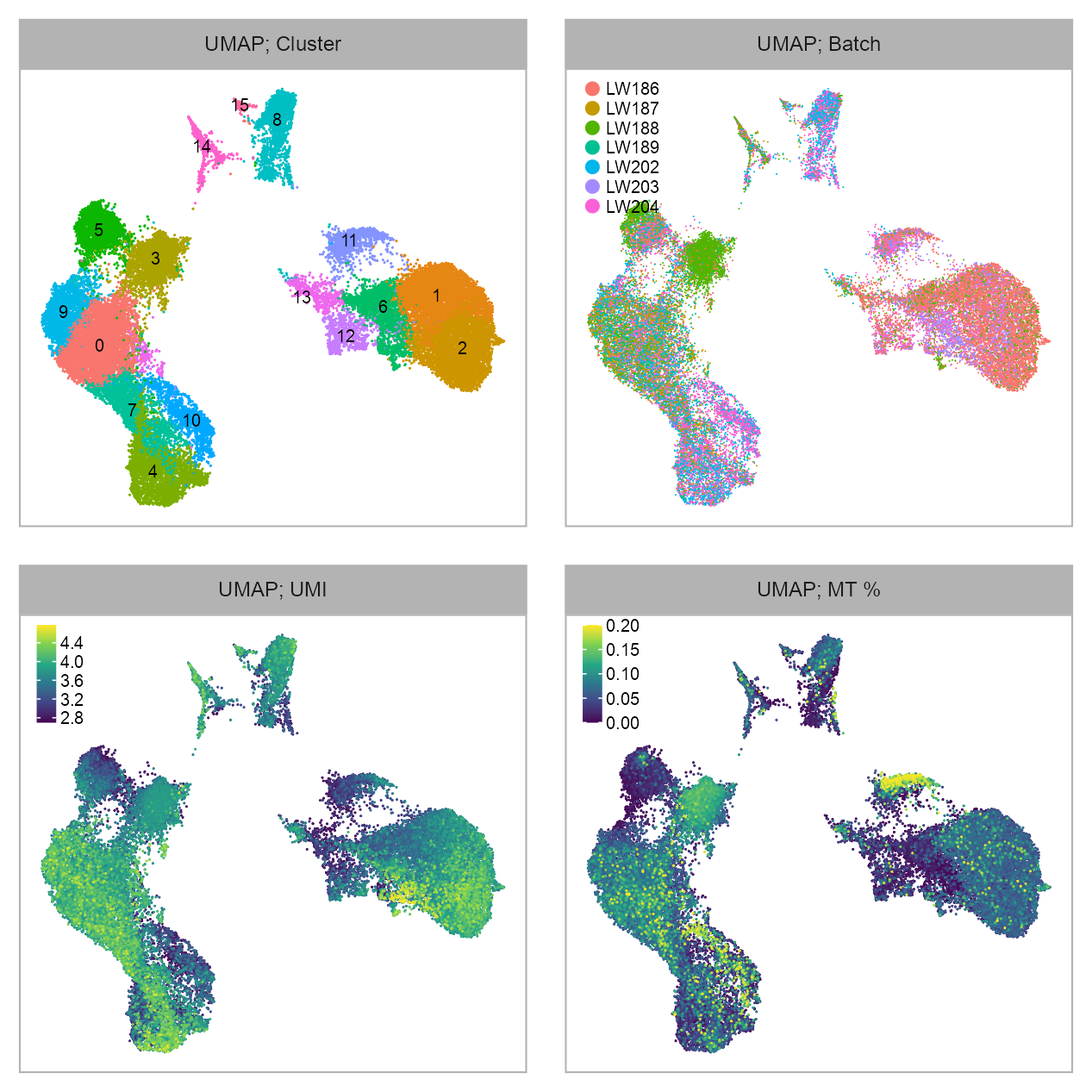
embedding_type <- EMBEDDING_TITLE_PREFIX

p_embedding_leiden <- plot_embedding(
    data = embedding[, c(x_column, y_column)],
    color = embedding$leiden |> as.factor(),
    label = glue::glue("{EMBEDDING_TITLE_PREFIX}; Cluster"),
    color_labels = TRUE,
    color_legend = FALSE,
    sort_values = FALSE,
    shuffle_values = TRUE,
    rasterise = RASTERISED,
    geom_point_size = GEOM_POINT_SIZE * 1.5
) +
    theme_customized_embedding()

p_embedding_batch <- plot_embedding(
    data = embedding[, c(x_column, y_column)],
    color = embedding$batch |> as.factor(),
    label = glue::glue("{EMBEDDING_TITLE_PREFIX}; Batch"),
    color_labels = FALSE,
    color_legend = TRUE,
    sort_values = FALSE,
    shuffle_values = TRUE,
    rasterise = RASTERISED,
    geom_point_size = GEOM_POINT_SIZE
) +
    theme_customized_embedding()

p_embedding_UMI <- plot_embedding(
    data = embedding[, c(x_column, y_column)],
    color = log10(Matrix::colSums(matrix_readcount_use[, embedding$cell])),
    label = glue::glue("{EMBEDDING_TITLE_PREFIX}; UMI"),
    color_legend = TRUE,
    sort_values = TRUE,
    shuffle_values = FALSE,
    rasterise = RASTERISED,
    geom_point_size = GEOM_POINT_SIZE * 1.5
) +
    theme_customized_embedding()

p_embedding_MT <- plot_embedding(
    data = embedding[, c(x_column, y_column)],
    color = embedding |>
        dplyr::left_join(cell_metadata, by = c("cell")) |>
        dplyr::pull(mt_percentage),
    label = glue::glue("{EMBEDDING_TITLE_PREFIX}; MT %"),
    color_legend = TRUE,
    sort_values = TRUE,
    shuffle_values = FALSE,
    rasterise = RASTERISED,
    geom_point_size = GEOM_POINT_SIZE * 1.5
) +
    theme_customized_embedding()

purrr::reduce(
    list(
        p_embedding_leiden,
        p_embedding_batch,
        p_embedding_UMI,
        p_embedding_MT
    ), `+`
) +
    patchwork::plot_layout(ncol = 2) +
    patchwork::plot_annotation(
        theme = ggplot2::theme(plot.margin = ggplot2::margin())
    )

cells_selected_stromal <- fs::dir_ls(
    file.path(
        PROJECT_DIR,
        "genotyping/result_vartrix_LW203_no-duplicates_umi_mapq10_consensus"
    )
) |>
    {
        \(x) {
            x[stringr::str_detect(
                string = x,
                pattern = "c*_stromal_snp*"
            )]
        }
    }() |>
    purrr::map(
        \(x) {
            scan(
                file = x, what = "charactor"
            )
        }
    ) |>
    unlist() |>
    unname() |>
    sort()

color_labels <- embedding[, c(x_column, y_column, "leiden")] |>
    dplyr::group_by(leiden) |>
    dplyr::summarise(
        x = median(.data[[x_column]]),
        y = median(.data[[y_column]]),
        .groups = "drop"
    ) |>
    as.data.frame()


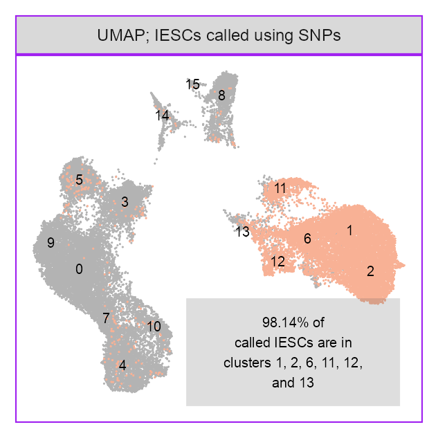
p_embedding_stromal <- plot_embedding(
    data = embedding[, c(x_column, y_column)],
    color = as.integer(embedding$cell %in% cells_selected_stromal) |> as.factor(),
    label = glue::glue("{EMBEDDING_TITLE_PREFIX}; IESCs called using SNPs"),
    color_labels = FALSE,
    color_legend = FALSE,
    sort_values = TRUE,
    shuffle_values = FALSE,
    rasterise = RASTERISED,
    geom_point_size = GEOM_POINT_SIZE * 1.5
) +
    theme_customized_embedding(
        panel_border_color = "purple",
        strip_background_fill = "#d9d9d9ff"
    ) +
    ggplot2::scale_color_manual(
        # values = c("grey70", "salmon")
        values = c("grey70", "#F8B195")
    )

p_embedding_stromal +
    ggplot2::annotate(
        geom = "text",
        x = color_labels[, "x"],
        y = color_labels[, "y"],
        label = color_labels[, 1],
        family = "Arial",
        color = "black",
        size = 5 / ggplot2::.pt,
        parse = TRUE
    ) +
    ggplot2::annotate(
        "rect",
        xmin = extract_ggplot2_axes_ranges(p_embedding_stromal)$x |>
            quantile(0.7) - 5.2,
        xmax = extract_ggplot2_axes_ranges(p_embedding_stromal)$x |>
            quantile(0.7) + 5.2,
        ymin = extract_ggplot2_axes_ranges(p_embedding_stromal)$y |>
            quantile(0.125) - 2.5,
        ymax = extract_ggplot2_axes_ranges(p_embedding_stromal)$y |>
            quantile(0.125) + 2.5,
        alpha = .2
    ) +
    ggplot2::annotate(
        geom = "text",
        # x = Inf,
        # y = Inf,
        x = extract_ggplot2_axes_ranges(p_embedding_stromal)$x |>
            quantile(0.7),
        y = extract_ggplot2_axes_ranges(p_embedding_stromal)$y |>
            quantile(0.125),
        label = glue::glue(
            "{scales::percent_format(accuracy = 0.01)(13617 / (13617 + 258))} of",
            "\ncalled IESCs ",
            "are in\nclusters 1, 2, 6, 11, 12,\nand 13"
        ),
        size = 5 / ggplot2::.pt,
        hjust = 0.5,
        vjust = 0.5,
        na.rm = FALSE,
        family = "Arial"
    )

color_palette_assay <- c(
    "Blastocyst (fibronectin)" = "#F28E2B",
    "Blastocyst (IESCs)" = "#4E79A7",
    "Blastoid (fibronectin)" = "#E15759",
    "Blastoid (IESCs)" = "#76B7B2",
    "IESCs" = "#59A14F"
)

embedding <- embedding |>
    dplyr::mutate(
        batch_annotated = dplyr::case_when(
            batch %in% c("LW187", "LW189") ~ "Blastocyst (fibronectin)",
            batch %in% c("LW186", "LW188") ~ "Blastocyst (IESCs)",
            batch %in% c("LW202") ~ "Blastoid (fibronectin)",
            batch %in% c("LW203") ~ "IESCs",
            batch %in% c("LW204") ~ "Blastoid (IESCs)"
        )
    )

Sample group

x_label <- extract_ggplot2_axes_ranges(p_embedding_leiden)$x |>
    unlist() |>
    quantile(0.78)

y_label <- extract_ggplot2_axes_ranges(p_embedding_leiden)$y |>
    unlist() |>
    quantile(0.99)

HJUST <- 0.5
VJUST <- 1

p_embedding_group <- list(
    plot_embedding(
        data = embedding[, c(x_column, y_column)],
        color = as.factor(embedding$leiden),
        # label = glue::glue("{EMBEDDING_TITLE_PREFIX}; Blastocyst"),
        color_labels = TRUE,
        color_legend = FALSE,
        # shape = values_shape,
        sort_values = FALSE,
        shuffle_values = TRUE,
        rasterise = RASTERISED,
        geom_point_size = GEOM_POINT_SIZE * 0.9,
        # geom_point_stroke = 0.125,
        geom_point_legend_ncol = 1
    ) +
        theme_customized_embedding(void = TRUE) +
        ggplot2::scale_color_manual(
            values = scales::hue_pal(
                l = 75, c = 150
            )(n = length(unique(embedding$leiden))),
            na.value = "grey70"
        ),
    #
    purrr::map(sort(unique(embedding$batch_annotated)), \(x) {
        plot_embedding(
            data = embedding[, c(x_column, y_column)],
            color = as.factor(as.integer(embedding$batch_annotated == x)),
            # label = glue::glue("{EMBEDDING_TITLE_PREFIX}; Blastocyst"),
            color_labels = FALSE,
            color_legend = FALSE,
            sort_values = TRUE,
            shuffle_values = FALSE,
            rasterise = RASTERISED,
            geom_point_size = GEOM_POINT_SIZE * 0.9,
            geom_point_legend_ncol = 1
        ) +
            theme_customized_embedding(
                void = TRUE
            ) +
            ggplot2::scale_color_manual(values = c("grey70", "salmon")) +
            ggplot2::annotate(
                geom = "text",
                x = x_label,
                y = y_label,
                label = x |>
                    stringr::str_replace(
                        pattern = " ",
                        replacement = "\n"
                    ),
                family = "Arial",
                color = "black",
                size = 5 / ggplot2::.pt,
                hjust = HJUST,
                vjust = VJUST
            )
    })
)

## | column: page
## | fig-width: 3.425195
## | fig-height: 1.427165

p_embedding_group |>
    purrr::reduce(`+`) +
    patchwork::plot_layout(
        nrow = 2,
        byrow = TRUE
    ) +
    patchwork::plot_annotation(
        theme = ggplot2::theme(plot.margin = ggplot2::margin())
    ) &
    theme_customized_clear()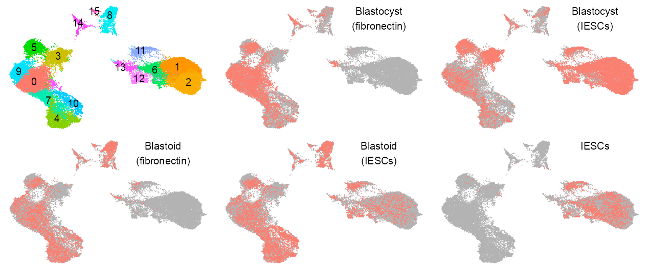

Expression

Embedding

features_selected <- c(
    "ENSG00000181449_SOX2",
    "ENSG00000164736_SOX17",
    #
    "ENSG00000179348_GATA2",
    "ENSG00000137869_CYP19A1",
    #
    "ENSG00000016082_ISL1",
    "ENSG00000134817_APLNR"
)

lineage_labels <- c(
    "(Epiblast)",
    "(Hypoblast)",
    "(Trophectoderm)",
    "(Trophectoderm)",
    "(Amnion)",
    "(Mesoderm)"
)

x_legend <- 0.0175
y_legend <- 0.995

num_columns <- 6
p_embedding_expression_lineage <- purrr::map2(
    features_selected, lineage_labels, \(x, y) {
        selected_feature <- x
        values <- log10(calc_cpm(matrix_readcount_use)[x, embedding$cell] + 1)
        # values[!embedding$cell %in% cells_blastoid_LW119_LW121] <- NA

        plot_embedding(
            data = embedding[, c(x_column, y_column)],
            color = values,
            # label = glue::glue(y),
            color_legend = TRUE,
            sort_values = TRUE,
            rasterise = RASTERISED,
            # geom_point_size = GEOM_POINT_SIZE * 0.7,
            geom_point_size = GEOM_POINT_SIZE * 0.9,
            na_value = "grey70"
        ) +
            theme_customized_embedding(
                x = x_legend,
                y = y_legend,
                void = TRUE,
                legend_key_size = c(1.2, 1.2)
            ) +
            ggplot2::annotate(
                geom = "text",
                x = x_label,
                y = y_label,
                label = stringr::str_c(
                    x |> stringr::str_remove(pattern = "^E.+_"),
                    y,
                    sep = "\n"
                ),
                family = "Arial",
                color = "black",
                size = 5 / ggplot2::.pt,
                hjust = HJUST,
                vjust = VJUST
            )
    }
)

features_selected <- c(
    "ENSG00000181350_LRRC75A",
    "ENSG00000143443_C1orf56",
    "ENSG00000118137_APOA1",
    #
    "ENSG00000189334_S100A14",
    "ENSG00000099953_MMP11",
    "ENSG00000111341_MGP"
)

num_columns <- 6
p_embedding_expression <- purrr::map(features_selected, \(x, y) {
    selected_feature <- x
    values <- log10(calc_cpm(matrix_readcount_use)[x, embedding$cell] + 1)
    # values[!embedding$cell %in% cells_blastoid_LW119_LW121] <- NA

    plot_embedding(
        data = embedding[, c(x_column, y_column)],
        color = values,
        # label = glue::glue(y),
        color_legend = TRUE,
        sort_values = TRUE,
        rasterise = RASTERISED,
        geom_point_size = GEOM_POINT_SIZE * 0.9,
        na_value = "grey70"
    ) +
        theme_customized_embedding(
            x = x_legend,
            y = y_legend,
            void = TRUE,
            legend_key_size = c(1.2, 1.2)
        ) +
        ggplot2::annotate(
            geom = "text",
            x = x_label,
            y = y_label,
            label = stringr::str_c(
                x |> stringr::str_remove(pattern = "^E.+_")
            ),
            family = "Arial",
            color = "black",
            size = 5 / ggplot2::.pt,
            hjust = HJUST,
            vjust = VJUST
        )
})

c(
    p_embedding_expression_lineage,
    p_embedding_expression
) |>
    purrr::reduce(`+`) +
    patchwork::plot_layout(
        nrow = 4,
        byrow = TRUE
    ) +
    patchwork::plot_annotation(
        theme = ggplot2::theme(plot.margin = ggplot2::margin())
    ) &
    theme_customized_clear()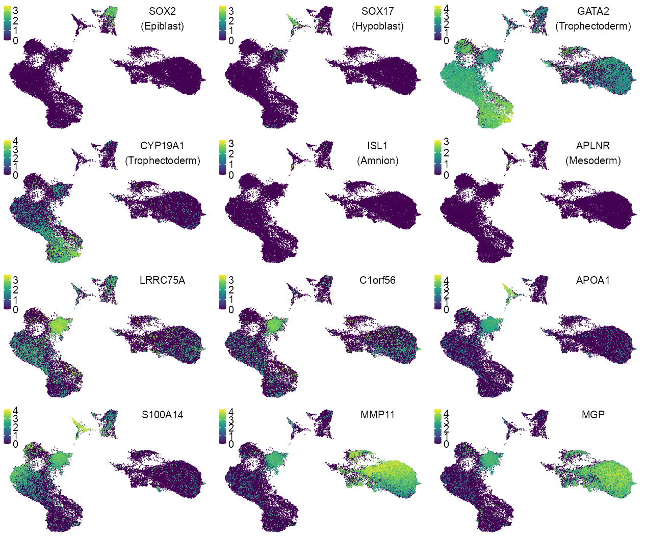

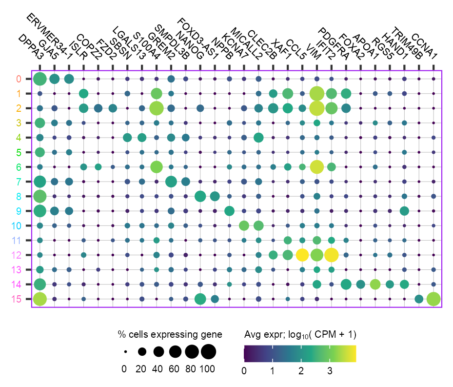
Lollipop

color_palette_leiden <- setNames(
    object = scales::hue_pal(l = 75, c = 150)(
        n = length(unique(embedding$leiden))
    ),
    nm = sort(unique(embedding$leiden))
)

features_selected <- c(
    "ENSG00000187569_DPPA3",
    "ENSG00000265107_GJA5",
    "ENSG00000226887_ERVMER34-1",
    "ENSG00000129009_ISLR",
    "ENSG00000005243_COPZ2",
    "ENSG00000180340_FZD2",
    "ENSG00000189001_SBSN",
    "ENSG00000105198_LGALS13",
    "ENSG00000196154_S100A4",
    "ENSG00000180875_GREM2",
    "ENSG00000130768_SMPDL3B",
    "ENSG00000111704_NANOG",
    "ENSG00000230798_FOXD3-AS1",
    "ENSG00000120937_NPPB",
    "ENSG00000104848_KCNA7",
    "ENSG00000164877_MICALL2",
    "ENSG00000110852_CLEC2B",
    "ENSG00000132530_XAF1",
    "ENSG00000271503_CCL5",
    "ENSG00000026025_VIM",
    "ENSG00000119922_IFIT2",
    "ENSG00000134853_PDGFRA",
    "ENSG00000125798_FOXA2",
    "ENSG00000118137_APOA1",
    "ENSG00000143248_RGS5",
    "ENSG00000113196_HAND1",
    "ENSG00000182053_TRIM49B",
    "ENSG00000026025_VIM",
    "ENSG00000133101_CCNA1"
) |>
    unique()

clusters_selected <- sort(unique(embedding$leiden)) |> as.character()

p_lollipop <- plot_lollipop(
    cells = (
        embedding |>
            split(~leiden) |>
            purrr::map(
                \(x) {
                    x |>
                        dplyr::filter(
                            batch %in% c("LW202", "LW204"),
                            !cell %in% cells_selected_stromal
                        ) |>
                        dplyr::pull(cell)
                }
            )
    )[clusters_selected],
    features = features_selected,
    matrix_cpm = calc_cpm(matrix_readcount_use),
    color_title = expression(paste("Avg expr; log"[10], "( CPM + 1)")),
    size_title = NULL
)

p_lollipop +
    ggplot2::scale_size(
        name = "% cells expressing gene",
        breaks = seq(0, 1, .2),
        labels = seq(0, 1, .2) * 100,
        limits = c(0, 1),
        range = c(0, 3),
        guide = ggplot2::guide_legend(
            title.position = "top",
            title.hjust = 0.5,
            label.position = "bottom",
            nrow = 1,
            byrow = TRUE,
            order = 1
        )
    ) +
    ggplot2::scale_color_viridis_c(
        name = expression(paste("Avg expr; log"[10], "( CPM + 1)")),
        guide = ggplot2::guide_colourbar(
            title.position = "top",
            title.hjust = 1,
            barwidth = 4,
            barheight = 0.6,
            direction = "horizontal",
            order = 2
        )
    ) +
    ggplot2::theme(
        axis.title.x = ggplot2::element_text(
            family = "Arial",
            size = 6,
            # margin = ggplot2::margin(t = 0, r = 0, b = 0, l = 0, unit = "mm")
        ),
        axis.title.y = ggplot2::element_text(
            family = "Arial",
            size = 6,
            # margin = ggplot2::margin(t = 0, r = 0, b = 0, l = 0, unit = "mm")
        ),
        axis.text.y = ggplot2::element_text(
            family = "Arial",
            color = rev(color_palette_leiden[as.character(clusters_selected)]),
            size = 5,
        ),
        axis.text.x = ggplot2::element_text(
            family = "Arial",
            color = "black",
            size = 5,
            angle = -45, vjust = 0.5, hjust = 1
        ),
        axis.line = ggplot2::element_blank(),
        #
        legend.background = ggplot2::element_blank(),
        legend.margin = ggplot2::margin(
            t = 0, r = 0, b = 0, l = 0, unit = "mm"
        ),
        legend.key = ggplot2::element_blank(),
        #
        legend.key.height = ggplot2::unit(2, "mm"),
        legend.key.width = ggplot2::unit(3, "mm"),
        #
        legend.position = "bottom",
        legend.box = "horizontal",
        #
        legend.text = ggplot2::element_text(
            family = "Arial",
            size = 5,
            margin = ggplot2::margin(
                t = 0, r = 0, b = 0, l = -0.5,
                unit = "mm"
            )
        ),
        legend.title = ggplot2::element_text(
            family = "Arial",
            size = 5
        ),
        #
        legend.box.background = ggplot2::element_blank(),
        #
        # panel.background = ggplot2::element_blank(),
        panel.background = ggplot2::element_rect(
            fill = NA, color = NA, linewidth = NULL
        ),
        panel.border = ggplot2::element_rect(
            fill = NA,
            color = "purple",
            linewidth = NULL
        ),
        panel.grid.major = ggplot2::element_line(
            color = "grey", linewidth = 0.125
        ),
        panel.grid.minor = ggplot2::element_blank(),
        #
        plot.background = ggplot2::element_blank(),
        plot.title = ggplot2::element_text(
            family = "Arial",
            size = 6,
            hjust = 0.5
        ),
    )

Composition

p_barplot_composition_leiden <- calc_group_composition(
    data = embedding,
    x = "leiden",
    group = "batch_annotated"
) |>
    dplyr::mutate(
        leiden = factor(leiden)
    ) |>
    dplyr::filter(
        # leiden %in% clusters_selected
    ) |>
    plot_barplot(
        x = "leiden",
        y = "percentage",
        z = "batch_annotated",
        legend_ncol = 1,
        #
        #
        axis_title_size = 5,
        axis_text_size = 5,
        legend_text_size = 5,
        #
        x_title = "Cluster; IESCs"
    ) +
    ggplot2::theme(
        panel.border = ggplot2::element_rect(
            fill = NA,
            color = "purple",
            linewidth = NULL
        ),
        axis.ticks = ggplot2::element_line(color = "black"),
        #
        axis.text.x = ggplot2::element_text(
            family = "Arial",
            # color = "black",
            color = scales::hue_pal(l = 75, c = 150)(
                n = length(unique(embedding$leiden))
            ),
            size = 5
        ),
    ) +
    ggplot2::scale_fill_manual(
        name = "Sample",
        values = color_palette_assay
    )

`summarise()` has grouped output by 'leiden'. You can override using the
`.groups` argument.

Warning: Vectorized input to `element_text()` is not officially supported.
ℹ Results may be unexpected or may change in future versions of ggplot2.

p_barplot_composition_leiden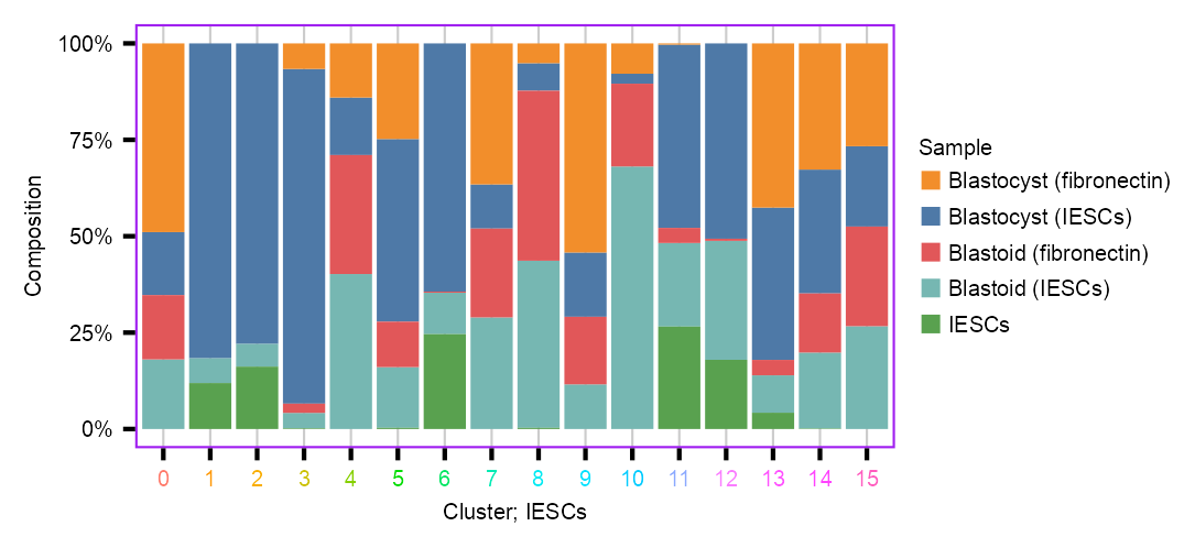

DE

prepare_features_to_mark <- function(d, num_features = 5) {
    purrr::map(names(d), \(x) {
        d[[x]] |>
            dplyr::mutate(
                category = x |>
                    stringr::str_remove(
                        pattern = "_.+$"
                    )
            ) |>
            tibble::rownames_to_column(var = "feature") |>
            dplyr::filter(
                fdr < 0.05,
            ) |>
            dplyr::mutate(
                group = dplyr::case_when(
                    log_fc > 0 ~ "up",
                    TRUE ~ "down"
                )
            ) |>
            split(~group) |>
            purrr::map(
                \(xx) {
                    xx |>
                        dplyr::arrange(desc(abs(log_fc))) |>
                        dplyr::slice(1:num_features)
                }
            ) |>
            dplyr::bind_rows() |>
            dplyr::mutate(
                name = stringr::str_remove(string = feature, pattern = "_.+$"),
                symbol = stringr::str_remove(string = feature, pattern = "^E.+_")
            )
    }) |>
        dplyr::bind_rows()
}

add_labels <- function(f) {
    ggrepel::geom_text_repel(
        data = f,
        ggplot2::aes(
            label = symbol,
        ),
        color = "black",
        size = 5 / ggplot2::.pt,
        family = "Arial",
        fontface = "plain",
        min.segment.length = -1e-10, box.padding = 0.5,
        segment.color = "grey30", # "grey70",
        segment.size = 0.25,
        segment.curvature = -10,
        segment.angle = 20,
        segment.ncp = 0,
        arrow = ggplot2::arrow(length = ggplot2::unit(0.0075, "npc")),
        #
        seed = 20220724 + 2023,
        max.iter = Inf,
        max.overlaps = Inf,
        nudge_x = 0,
        nudge_y = 0,
        point.padding = 0,
        #
        hjust = 0
    )
}

theme_customized_scatter <- function() {
    ggplot2::theme(
        axis.title.x = ggplot2::element_text(
            family = "Arial",
            size = 5,
        ),
        axis.title.y = ggplot2::element_text(
            family = "Arial",
            size = 5,
            margin = ggplot2::margin(t = 0, r = 0, b = 0, l = 0, unit = "mm")
        ),
        axis.text = ggplot2::element_text(
            family = "Arial",
            color = "black",
            size = 5
        ),
        #
        plot.title = ggplot2::element_text(
            family = "Arial",
            size = 6,
            hjust = 0.5,
            margin = ggplot2::margin(t = 0, r = 0, b = 1, l = 0, unit = "mm")
        ),
        strip.text = ggplot2::element_text(
            family = "Arial", size = 5
        ),
        panel.border = ggplot2::element_rect(
            fill = NA, color = "purple",
        ),
        strip.background = ggplot2::element_rect(
            fill = "#d9d9d9ff", color = "purple"
        )
    )
}

EDGER_METHOD <- "lrt"
LOG_FC_THRESHOLD <- 1

Blastocyst vs. blastoid

clusters_selected <- list(
    ELCs = c(8),
    HLCs = c(14),
    TLCs = c(0, 3, 4, 5, 7, 9, 10)
)

de <- purrr::map(names(clusters_selected), \(x) {
    cells_1 <- embedding |>
        dplyr::filter(
            leiden %in% clusters_selected[[x]],
            !cell %in% cells_selected_stromal,
            batch %in% c("LW186", "LW188", "LW187", "LW189")
        ) |>
        dplyr::pull(cell)

    cells_2 <- embedding |>
        dplyr::filter(
            leiden %in% clusters_selected[[x]],
            !cell %in% cells_selected_stromal,
            batch %in% c("LW204", "LW202")
        ) |>
        dplyr::pull(cell)

    cat(x, length(cells_1), length(cells_2), "\n")

    # if (length(cells_1) >= 100 & length(cells_2) >= 100) {
    out <- run_pseudobulk_edgeR(
        matrix = matrix_readcount_use,
        cells_1 = cells_1,
        cells_2 = cells_2,
        method = EDGER_METHOD,
        log_fc_threshold = LOG_FC_THRESHOLD
    )
    # } else {
    #    out <- NULL
    # }
    return(out)
})

ELCs 269 1963

number of pseudobulks: 8 (269) vs 10 (1963)

HLCs 530 284

number of pseudobulks: 9 (530) vs 9 (284)

TLCs 12707 8340

number of pseudobulks: 10 (12707) vs 9 (8340)

names(de) <- names(clusters_selected)

de <- purrr::map(de, \(x) {
    x$edgeR_result
})

features_to_mark <- prepare_features_to_mark(de)

p_scatter_de <- purrr::map(names(de), \(x) {
    de[[x]] |>
        dplyr::mutate(
            category = x |>
                stringr::str_remove(
                    pattern = "_.+$"
                )
        ) |>
        tibble::rownames_to_column(var = "feature")
}) |>
    dplyr::bind_rows() |>
    dplyr::mutate(
        de = dplyr::case_when(
            fdr < 0.05 & abs(log_fc) >= 2 ~ "1",
            TRUE ~ "0"
        )
    ) |>
    ggplot2::ggplot(
        aes(
            x = log_cpm,
            y = log_fc,
            color = de
        )
    ) +
    ggrastr::rasterise(
        input = ggplot2::geom_point(alpha = 0.8, size = 0.8, stroke = 0),
        dpi = 900,
        dev = "ragg_png"
    ) +
    ggplot2::facet_grid(cols = vars(category), scales = "free")

p_scatter_de <- p_scatter_de +
    ggplot2::scale_color_manual(values = c("grey70", "#00BFC4")) +
    ggplot2::scale_x_continuous(
        name = expression(paste("Average CPM ", "(log"[2], ")")),
    ) +
    ggplot2::scale_y_continuous(
        name = expression(paste("Fold change ", "(log"[2], ")")),
    ) +
    ggplot2::ggtitle(label = "Blastocyst vs. blastoid") +
    ggplot2::guides(color = "none") +
    theme_customized2() +
    theme_customized_scatter() # + add_labels(features_to_mark)

g <- ggplot2::ggplot_gtable(
    ggplot2::ggplot_build(p_scatter_de)
)
stript <- which(grepl("strip-t", g$layout$name))


k <- 1
for (i in stript) {
    j <- which(grepl("rect", g$grobs[[i]]$grobs[[1]]$childrenOrder))
    g$grobs[[i]]$grobs[[1]]$children[[j]]$gp$fill <- setNames(
        object = c(ELCs = "#8ace7e", HLCs = "#ff684c", TLCs = "#9467bd"),
        nm = seq_len(3)
    )[k]
    k <- k + 1
}
grid::grid.draw(g)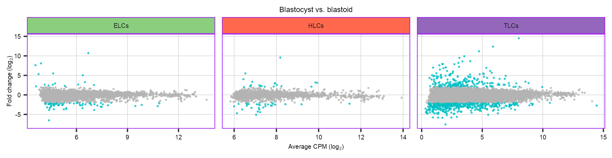

Clusters 3-5 vs. 0-7-9

clusters_selected_1 <- c(3, 5)
clusters_selected_2 <- c(0, 7, 9)

cells_1 <- embedding |>
    dplyr::filter(
        leiden %in% clusters_selected_1,
        !batch %in% c("LW203")
    ) |>
    dplyr::pull(cell)


cells_2 <- embedding |>
    dplyr::filter(
        leiden %in% clusters_selected_2,
        !batch %in% c("LW203")
    ) |>
    dplyr::pull(cell)

cat(length(cells_1), length(cells_2), "\n")

6645 9817

de <- run_pseudobulk_edgeR(
    matrix = matrix_readcount_use,
    cells_1 = cells_1,
    cells_2 = cells_2,
    method = EDGER_METHOD,
    log_fc_threshold = LOG_FC_THRESHOLD
)

number of pseudobulks: 10 (6645) vs 10 (9817)

# de <- de$edgeR_result

features_to_mark <- de$edgeR_result |>
    tibble::rownames_to_column(var = "feature") |>
    dplyr::mutate(
        symbol = stringr::str_remove_all(
            string = feature,
            pattern = "^E.+_"
        )
    ) |>
    dplyr::filter(
        symbol %in% c(
            "MMP10",
            "MMP3",
            "CTGF",
            "KRT17",
            "CNN1",
            "SERPINE2",
            "FN1",
            "DBP"
        )
    )

p_scatter_de <- de$edgeR_result |>
    tibble::rownames_to_column(var = "feature") |>
    dplyr::mutate(
        de = dplyr::case_when(
            fdr < 0.05 & abs(log_fc) >= 1 ~ "1",
            TRUE ~ "0"
        )
    ) |>
    dplyr::arrange((de)) |>
    ggplot2::ggplot(
        aes(
            x = log_cpm,
            y = log_fc,
            color = de
        )
    ) +
    ggrastr::rasterise(
        input = ggplot2::geom_point(alpha = 0.8, size = 0.8, stroke = 0),
        dpi = 900,
        dev = "ragg_png"
    )

p_scatter_de +
    ggplot2::scale_color_manual(values = c("grey70", "#00BFC4")) +
    ggplot2::scale_x_continuous(
        name = expression(paste("Average CPM ", "(log"[2], ")")),
    ) +
    ggplot2::scale_y_continuous(
        name = expression(paste("Fold change ", "(log"[2], ")")),
        limits = c(-4, 5.862482)
    ) +
    ggplot2::ggtitle(label = "Cluster 3-5 vs. 0-7-9") +
    ggplot2::guides(color = "none") +
    theme_customized2() +
    theme_customized_scatter() +
    add_labels(features_to_mark)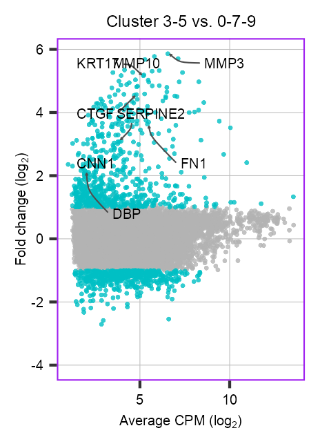

Gene Ontology enrichment

plot_barplot_go <- function(x, x_title) {
    ggplot2::ggplot(
        data = x,
        ggplot2::aes(
            x = -log10(p_value),
            y = as.factor(rev(rank))
        )
    ) +
        ggplot2::geom_bar(
            stat = "identity",
            fill = "#707d75",
            alpha = 0.8
        ) +
        ggplot2::scale_x_continuous(
            # name = expression(paste("Cluster 0-7-9; -log"[10], " p", sep = "")),
            name = x_title,
            labels = scales::math_format(10^.x)
        ) +
        ggplot2::guides(fill = "none") +
        ggplot2::geom_text(
            ggplot2::aes(
                x = 0,
                label = paste(" ", term, sep = ""),
                group = NULL
            ),
            size = 6 / ggplot2::.pt,
            family = "Arial",
            color = "black",
            data = x,
            hjust = 0
        ) +
        ggplot2::theme_classic() +
        ggplot2::theme(
            axis.title.x = ggplot2::element_text(family = "Arial", size = 5),
            axis.title.y = ggplot2::element_blank(),
            axis.text.x = ggplot2::element_text(family = "Arial", size = 5),
            axis.text.y = ggplot2::element_blank(),
            axis.ticks.y = ggplot2::element_blank(),
            axis.line.y = ggplot2::element_blank(),
            legend.text = ggplot2::element_text(family = "Arial", size = 5),
            legend.title = ggplot2::element_text(family = "Arial", size = 5)
        ) +
        ggplot2::theme(
            axis.line.x.bottom = element_line(color = "purple", linewidth = 0.3),
            panel.background = ggplot2::element_blank(),
            plot.background = ggplot2::element_blank()
        )
}

enriched_go <- tibble::tribble(
    ~go_id, ~term, ~p_value,
    "GO:0030198", "extracellular matrix organization", 1.6e-18,
    "GO:0045229", "external encapsulating structure organization", 2.5e-18,
    "GO:0001944", "vasculature development", 1e-16,
    "GO:0001568", "blood vessel development", 1.3e-16,
    "GO:0030199", "collagen fibril organization", 1.4e-15,
    "GO:0016477", "cell migration", 2e-16,
    "GO:0032963", "collagen metabolic process", 6.1e-21,
    "GO:0009653", "anatomical structure morphogenesis", 2.8e-15,
    "GO:0048514", "blood vessel morphogenesis", 3.2e-14,
    "GO:0072359", "circulatory system development", 8e-15,
    "GO:0097435", "supramolecular fiber organization", 7.4e-14,
    "GO:0035295", "tube development", 2.3e-13
) |>
    dplyr::mutate(
        p_value_log = -log10(p_value),
        term = stringr::str_replace_all(
            string = term,
            pattern = "organization0",
            replacement = "org."
        )
    ) |>
    dplyr::arrange(
        p_value
    ) |>
    dplyr::mutate(rank = 1:dplyr::n())

p_barplot_go_bp_3_5 <- plot_barplot_go(
    enriched_go,
    x_title = expression(paste("Cluster 3-5; -log"[10], " p", sep = ""))
)

enriched_go <- tibble::tribble(
    ~go_id, ~term, ~p_value,
    "GO:0051276", "chromosome organization", 1.3e-16,
    "GO:0090304", "nucleic acid metabolic process", 6.2e-16,
    "GO:0006139", "nucleobase-containing compound metabolic process", 1.3e-12,
    "GO:0097659", "nucleic acid-templated transcription", 1.1e-13,
    "GO:0032774", "RNA biosynthetic process", 1.8e-13,
    "GO:0006351", "transcription, DNA-templated", 2.3e-13,
    "GO:0051252", "regulation of RNA metabolic process", 8.3e-13,
    "GO:0006996", "organelle organization", 3.8e-12,
    "GO:0046483", "heterocycle metabolic process", 4.3e-12,
    "GO:0019438", "aromatic compound biosynthetic process", 5.2e-12,
    "GO:0006725", "cellular aromatic compound metabolic process", 7.2e-12,
    "GO:0016570", "histone modification", 8e-12
) |>
    dplyr::arrange(p_value) |>
    dplyr::mutate(
        p_value_log = -log10(p_value),
        term = stringr::str_replace_all(
            string = term,
            pattern = "organization0",
            replacement = "org."
        )
    ) |>
    dplyr::arrange(
        p_value
    ) |>
    dplyr::mutate(rank = 1:dplyr::n())

p_barplot_go_bp_0_7_9 <- plot_barplot_go(
    enriched_go,
    x_title = expression(paste("Cluster 0-7-9; -log"[10], " p", sep = ""))
)

list(
    p_barplot_go_bp_3_5,
    p_barplot_go_bp_0_7_9
) |>
    purrr::reduce(`+`) +
    patchwork::plot_layout(nrow = 1) +
    patchwork::plot_annotation(
        theme = theme(plot.margin = margin())
    ) &
    theme_customized_clear()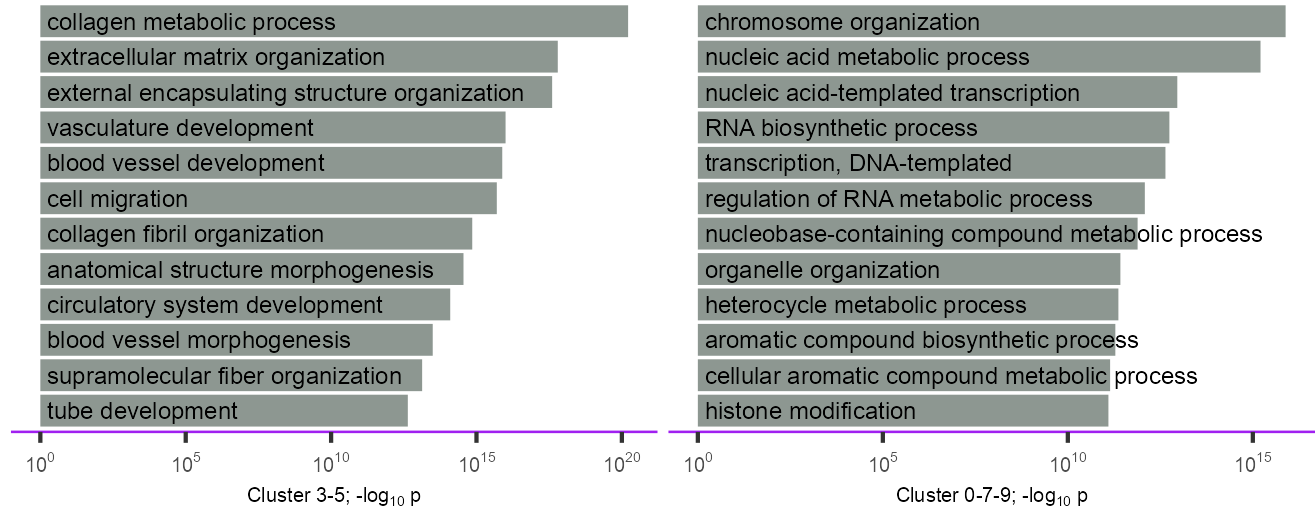

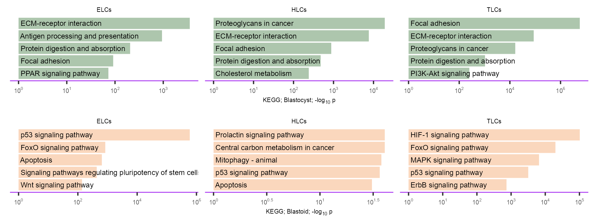
KEGG enrichment

enriched_kegg <- tibble::tribble(
    ~id, ~description, ~GeneRatio, ~BgRatio, ~pvalue, ~category, ~group,
    "hsa04512", "ECM-receptor interaction", "5/42", "88/6234", 0.000281855, "ELCs", "blastocyst",
    "hsa04612", "Antigen processing and presentation", "4/42", "68/6234", 0.001060988, "ELCs", "blastocyst",
    "hsa04974", "Protein digestion and absorption", "4/42", "103/6234", 0.004859407, "ELCs", "blastocyst",
    "hsa04510", "Focal adhesion", "5/42", "202/6234", 0.010913578, "ELCs", "blastocyst",
    "hsa03320", "PPAR signaling pathway", "3/42", "75/6234", 0.013720541, "ELCs", "blastocyst",
    "hsa05205", "Proteoglycans in cancer", "11/81", "202/6234", 5.22765e-05, "HLCs", "blastocyst",
    "hsa04512", "ECM-receptor interaction", "7/81", "88/6234", 0.000130988, "HLCs", "blastocyst",
    "hsa04510", "Focal adhesion", "9/81", "202/6234", 0.001139082, "HLCs", "blastocyst",
    "hsa04974", "Protein digestion and absorption", "6/81", "103/6234", 0.002095322, "HLCs", "blastocyst",
    "hsa04979", "Cholesterol metabolism", "4/81", "51/6234", 0.004159024, "HLCs", "blastocyst",
    "hsa04510", "Focal adhesion", "28/292", "202/6234", 1.7399e-07, "TLCs", "blastocyst",
    "hsa04512", "ECM-receptor interaction", "15/292", "88/6234", 1.14579e-05, "TLCs", "blastocyst",
    "hsa05205", "Proteoglycans in cancer", "23/292", "202/6234", 6.13288e-05, "TLCs", "blastocyst",
    "hsa04974", "Protein digestion and absorption", "13/292", "103/6234", 0.000958324, "TLCs", "blastocyst",
    "hsa04151", "PI3K-Akt signaling pathway", "28/292", "353/6234", 0.003988003, "TLCs", "blastocyst",
    "hsa04115", "p53 signaling pathway", "10/126", "73/6234", 1.68217e-06, "ELCs", "blastoid",
    "hsa04068", "FoxO signaling pathway", "9/126", "130/6234", 0.001188586, "ELCs", "blastoid",
    "hsa04210", "Apoptosis", "9/126", "135/6234", 0.001550454, "ELCs", "blastoid",
    "hsa04550", "Signaling pathways regulating pluripotency of stem cells", "9/126", "143/6234", 0.002309383, "ELCs", "blastoid",
    "hsa04310", "Wnt signaling pathway", "9/126", "170/6234", 0.00724, "ELCs", "blastoid",
    "hsa04917", "Prolactin signaling pathway", "3/56", "70/6234", 0.024598088, "HLCs", "blastoid",
    "hsa05230", "Central carbon metabolism in cancer", "3/56", "70/6234", 0.024598088, "HLCs", "blastoid",
    "hsa04137", "Mitophagy - animal", "3/56", "72/6234", 0.026466658, "HLCs", "blastoid",
    "hsa04115", "p53 signaling pathway", "3/56", "73/6234", 0.027428868, "HLCs", "blastoid",
    "hsa04210", "Apoptosis", "4/56", "135/6234", 0.032458563, "HLCs", "blastoid",
    "hsa04066", "HIF-1 signaling pathway", "21/422", "109/6234", 9.77485e-06, "TLCs", "blastoid",
    "hsa04068", "FoxO signaling pathway", "22/422", "130/6234", 5.04122e-05, "TLCs", "blastoid",
    "hsa04010", "MAPK signaling pathway", "37/422", "294/6234", 0.000152211, "TLCs", "blastoid",
    "hsa04115", "p53 signaling pathway", "14/422", "73/6234", 0.000314539, "TLCs", "blastoid",
    "hsa04012", "ErbB signaling pathway", "14/422", "84/6234", 0.001361888, "TLCs", "blastoid"
)

purrr::map2(c("Blastocyst", "Blastoid"), c("#99B898", "#F9CDAD"), \(x, y) {
    enriched_kegg |>
        dplyr::mutate(
            group = stringr::str_to_title(group)
        ) |>
        dplyr::select(
            go_id = id,
            term = description,
            p_value = pvalue,
            category,
            group
        ) |>
        dplyr::filter(group == x) |>
        split(~category) |>
        purrr::map(
            \(x)
            x |>
                dplyr::arrange(p_value) |>
                dplyr::slice(1:5) |>
                dplyr::mutate(rank = 1:dplyr::n())
        ) |>
        dplyr::bind_rows() |>
        dplyr::mutate(
            p_value_log = -log10(p_value)
        ) |>
        {
            \(z) {
                z |>
                    ggplot2::ggplot(
                        ggplot2::aes(
                            x = -log10(p_value),
                            y = as.factor(rev(rank))
                        )
                    ) +
                    ggplot2::geom_bar(
                        stat = "identity",
                        fill = y,
                        alpha = 0.8
                    ) +
                    ggplot2::facet_grid(
                        cols = ggplot2::vars(category), scales = "free_x"
                    ) +
                    ggplot2::scale_x_continuous(
                        name = glue::glue(
                            "KEGG; {x}; -log<sub>10</sub> p"
                        ),
                        labels = scales::math_format(10^.x)
                    ) +
                    ggplot2::guides(fill = "none") +
                    ggplot2::geom_text(
                        ggplot2::aes(
                            x = 0,
                            label = paste(" ", term, sep = ""),
                            group = NULL
                        ),
                        size = 6 / ggplot2::.pt,
                        family = "Arial",
                        color = "black",
                        data = z,
                        hjust = 0
                    ) +
                    ggplot2::theme(
                        axis.title.x = ggplot2::element_text(
                            family = "Arial", size = 5
                        ),
                        axis.title.y = ggplot2::element_blank(),
                        axis.text.x = ggplot2::element_text(
                            family = "Arial", size = 5
                        ),
                        axis.text.y = ggplot2::element_blank(),
                        axis.ticks.y = ggplot2::element_blank(),
                        axis.line.y = ggplot2::element_blank(),
                        legend.text = ggplot2::element_text(
                            family = "Arial", size = 5
                        ),
                        legend.title = ggplot2::element_text(
                            family = "Arial", size = 5
                        )
                    ) +
                    ggplot2::theme(
                        axis.line.x.bottom = ggplot2::element_line(
                            color = "purple", linewidth = 0.3
                        ),
                        panel.background = ggplot2::element_blank(),
                        plot.background = ggplot2::element_blank(),
                        #
                        strip.background = ggplot2::element_rect(
                            fill = NA,
                            color = NA
                        ),
                        #
                        strip.text = ggplot2::element_text(
                            family = "Arial",
                            size = 5,
                            color = "black",
                            hjust = 0.5,
                            margin = ggplot2::margin(
                                t = 0, r = 0, b = 1, l = 0,
                                unit = "mm"
                            )
                        ),
                        axis.title.x = ggtext::element_markdown(),
                    )
            }
        }()
}) |>
    purrr::reduce(`+`) +
    patchwork::plot_layout(ncol = 1, byrow = FALSE) +
    patchwork::plot_annotation(
        theme = ggplot2::theme(plot.margin = ggplot2::margin())
    )

R session info

devtools::session_info()

─ Session info ───────────────────────────────────────────────────────────────
 setting  value
 version  R version 4.3.1 (2023-06-16)
 os       macOS Ventura 13.5.2
 system   aarch64, darwin22.4.0
 ui       unknown
 language (EN)
 collate  en_US.UTF-8
 ctype    en_US.UTF-8
 tz       America/Chicago
 date     2023-09-10
 pandoc   2.19.2 @ /Users/jialei/.pyenv/shims/ (via rmarkdown)

─ Packages ───────────────────────────────────────────────────────────────────
 package     * version     date (UTC) lib source
 beeswarm      0.4.0       2021-06-01 [1] CRAN (R 4.3.0)
 bit           4.0.5       2022-11-15 [1] CRAN (R 4.3.0)
 bit64         4.0.5       2020-08-30 [1] CRAN (R 4.3.0)
 cachem        1.0.8       2023-05-01 [1] CRAN (R 4.3.0)
 callr         3.7.3       2022-11-02 [1] CRAN (R 4.3.0)
 cli           3.6.1       2023-03-23 [1] CRAN (R 4.3.0)
 colorspace    2.1-0       2023-01-23 [1] CRAN (R 4.3.0)
 commonmark    1.9.0       2023-03-17 [1] CRAN (R 4.3.0)
 crayon        1.5.2       2022-09-29 [1] CRAN (R 4.3.0)
 devtools      2.4.5.9000  2023-08-11 [1] Github (r-lib/devtools@163c3f2)
 digest        0.6.33      2023-07-07 [1] CRAN (R 4.3.1)
 dplyr       * 1.1.3       2023-09-03 [1] CRAN (R 4.3.1)
 ellipsis      0.3.2       2021-04-29 [1] CRAN (R 4.3.0)
 evaluate      0.21        2023-05-05 [1] CRAN (R 4.3.0)
 extrafont   * 0.19        2023-01-18 [1] CRAN (R 4.3.0)
 extrafontdb   1.0         2012-06-11 [1] CRAN (R 4.3.0)
 fansi         1.0.4       2023-01-22 [1] CRAN (R 4.3.0)
 farver        2.1.1       2022-07-06 [1] CRAN (R 4.3.0)
 fastmap       1.1.1       2023-02-24 [1] CRAN (R 4.3.0)
 forcats     * 1.0.0.9000  2023-04-23 [1] Github (tidyverse/forcats@4a8525a)
 fs            1.6.3       2023-07-20 [1] CRAN (R 4.3.1)
 generics      0.1.3       2022-07-05 [1] CRAN (R 4.3.0)
 ggbeeswarm    0.7.2       2023-04-29 [1] CRAN (R 4.3.0)
 ggplot2     * 3.4.3.9000  2023-09-05 [1] Github (tidyverse/ggplot2@d180248)
 ggrastr       1.0.2       2023-06-01 [1] CRAN (R 4.3.0)
 ggrepel       0.9.3       2023-02-03 [1] CRAN (R 4.3.0)
 ggtext        0.1.2       2022-09-16 [1] CRAN (R 4.3.0)
 glue          1.6.2.9000  2023-04-23 [1] Github (tidyverse/glue@cbac82a)
 gridtext      0.1.5       2022-09-16 [1] CRAN (R 4.3.0)
 gt            0.9.0.9000  2023-09-02 [1] Github (rstudio/gt@c73eece)
 gtable        0.3.4.9000  2023-08-22 [1] Github (r-lib/gtable@c410a54)
 hms           1.1.3       2023-03-21 [1] CRAN (R 4.3.0)
 htmltools     0.5.6       2023-08-10 [1] CRAN (R 4.3.1)
 htmlwidgets   1.6.2       2023-03-17 [1] CRAN (R 4.3.0)
 jsonlite      1.8.7       2023-06-29 [1] CRAN (R 4.3.1)
 knitr         1.43        2023-05-25 [1] CRAN (R 4.3.0)
 labeling      0.4.3       2023-08-29 [1] CRAN (R 4.3.1)
 lattice       0.21-8      2023-04-05 [2] CRAN (R 4.3.1)
 lifecycle     1.0.3       2022-10-07 [1] CRAN (R 4.3.0)
 lubridate   * 1.9.2.9000  2023-07-22 [1] Github (tidyverse/lubridate@cae67ea)
 magrittr      2.0.3       2022-03-30 [1] CRAN (R 4.3.0)
 markdown      1.8         2023-08-23 [1] CRAN (R 4.3.1)
 Matrix      * 1.6-1       2023-08-14 [2] CRAN (R 4.3.1)
 memoise       2.0.1       2021-11-26 [1] CRAN (R 4.3.0)
 munsell       0.5.0       2018-06-12 [1] CRAN (R 4.3.0)
 patchwork   * 1.1.3.9000  2023-08-17 [1] Github (thomasp85/patchwork@51a6eff)
 pillar        1.9.0       2023-03-22 [1] CRAN (R 4.3.0)
 pkgbuild      1.4.2       2023-06-26 [1] CRAN (R 4.3.1)
 pkgconfig     2.0.3       2019-09-22 [1] CRAN (R 4.3.0)
 pkgload       1.3.2.9000  2023-07-05 [1] Github (r-lib/pkgload@3cf9896)
 png           0.1-8       2022-11-29 [1] CRAN (R 4.3.0)
 prettyunits   1.1.1.9000  2023-04-23 [1] Github (r-lib/prettyunits@8706d89)
 processx      3.8.2       2023-06-30 [1] CRAN (R 4.3.1)
 ps            1.7.5       2023-04-18 [1] CRAN (R 4.3.0)
 purrr       * 1.0.2.9000  2023-08-11 [1] Github (tidyverse/purrr@ac4f5a9)
 R.cache       0.16.0      2022-07-21 [1] CRAN (R 4.3.0)
 R.methodsS3   1.8.2       2022-06-13 [1] CRAN (R 4.3.0)
 R.oo          1.25.0      2022-06-12 [1] CRAN (R 4.3.0)
 R.utils       2.12.2      2022-11-11 [1] CRAN (R 4.3.0)
 R6            2.5.1.9000  2023-04-23 [1] Github (r-lib/R6@e97cca7)
 ragg          1.2.5       2023-01-12 [1] CRAN (R 4.3.0)
 Rcpp          1.0.11      2023-07-06 [1] CRAN (R 4.3.1)
 readr       * 2.1.4.9000  2023-08-03 [1] Github (tidyverse/readr@80e4dc1)
 remotes       2.4.2.9000  2023-06-09 [1] Github (r-lib/remotes@8875171)
 reticulate    1.31        2023-08-10 [1] CRAN (R 4.3.1)
 rlang         1.1.1.9000  2023-06-09 [1] Github (r-lib/rlang@c55f602)
 rmarkdown     2.24.2      2023-09-07 [1] Github (rstudio/rmarkdown@8d2d9b8)
 rstudioapi    0.15.0.9000 2023-09-07 [1] Github (rstudio/rstudioapi@19c80c0)
 Rttf2pt1      1.3.12      2023-01-22 [1] CRAN (R 4.3.0)
 sass          0.4.7       2023-07-15 [1] CRAN (R 4.3.1)
 scales        1.2.1       2022-08-20 [1] CRAN (R 4.3.0)
 sessioninfo   1.2.2       2021-12-06 [1] CRAN (R 4.3.0)
 stringi       1.7.12      2023-01-11 [1] CRAN (R 4.3.0)
 stringr     * 1.5.0.9000  2023-08-11 [1] Github (tidyverse/stringr@08ff36f)
 styler      * 1.10.2      2023-08-30 [1] Github (r-lib/styler@1976817)
 systemfonts   1.0.4       2022-02-11 [1] CRAN (R 4.3.0)
 textshaping   0.3.6       2021-10-13 [1] CRAN (R 4.3.0)
 tibble      * 3.2.1.9005  2023-05-28 [1] Github (tidyverse/tibble@4de5c15)
 tidyr       * 1.3.0.9000  2023-04-23 [1] Github (tidyverse/tidyr@0764e65)
 tidyselect    1.2.0       2022-10-10 [1] CRAN (R 4.3.0)
 tidyverse   * 2.0.0.9000  2023-04-23 [1] Github (tidyverse/tidyverse@8ec2e1f)
 timechange    0.2.0       2023-01-11 [1] CRAN (R 4.3.0)
 tzdb          0.4.0       2023-05-12 [1] CRAN (R 4.3.0)
 usethis       2.2.2.9000  2023-07-11 [1] Github (r-lib/usethis@467ff57)
 utf8          1.2.3       2023-01-31 [1] CRAN (R 4.3.0)
 vctrs         0.6.3       2023-06-14 [1] CRAN (R 4.3.0)
 vipor         0.4.5       2017-03-22 [1] CRAN (R 4.3.0)
 viridisLite   0.4.2       2023-05-02 [1] CRAN (R 4.3.0)
 vroom         1.6.3.9000  2023-04-30 [1] Github (tidyverse/vroom@89b6aac)
 withr         2.5.0       2022-03-03 [1] CRAN (R 4.3.0)
 xfun          0.40        2023-08-09 [1] CRAN (R 4.3.1)
 xml2          1.3.5       2023-07-06 [1] CRAN (R 4.3.1)
 yaml          2.3.7       2023-01-23 [1] CRAN (R 4.3.0)

 [1] /opt/homebrew/lib/R/4.3/site-library
 [2] /opt/homebrew/Cellar/r/4.3.1/lib/R/library

─ Python configuration ───────────────────────────────────────────────────────
 python:         /Users/jialei/.pyenv/shims/python
 libpython:      /Users/jialei/.pyenv/versions/mambaforge-22.9.0-3/lib/libpython3.10.dylib
 pythonhome:     /Users/jialei/.pyenv/versions/mambaforge-22.9.0-3:/Users/jialei/.pyenv/versions/mambaforge-22.9.0-3
 version:        3.10.9 | packaged by conda-forge | (main, Feb  2 2023, 20:26:08) [Clang 14.0.6 ]
 numpy:          /Users/jialei/.pyenv/versions/mambaforge-22.9.0-3/lib/python3.10/site-packages/numpy
 numpy_version:  1.24.3
 numpy:          /Users/jialei/.pyenv/versions/mambaforge-22.9.0-3/lib/python3.10/site-packages/numpy
 
 NOTE: Python version was forced by RETICULATE_PYTHON

──────────────────────────────────────────────────────────────────────────────

Styling  1  files:
 interpret_blastoids_stromal.qmd ✔ 
────────────────────────────────────────
Status  Count   Legend 
✔   1   File unchanged.
ℹ   0   File changed.
✖   0   Styling threw an error.
────────────────────────────────────────